Evaluation of predictions of the stochastic model of organelle production based on exact distributions
- University of Sheffield, United Kingdom
Figures
Figure 1

The concept of the limiting distribution in a stochastic system.
(A) The traces show simulations run with the parameters {kde novo = 2.0, kfission = 0.9; γ = 1.0, kfusion = 0.02}, starting from n = 0 (black trace) and n = 50 (green trace). Both simulations “settle down” to stochastic fluctuations about a mean value of <n> = 7.1 (B) Schematic representation of a set of cells that are all initialised to n = 1 at time t = 0, and are observed at a time t = τ. (C) Distributions calculated with the same parameters as in (A) for a set of 1000 cells as in (B), calculated for τ = 0.2 (magenta), 0.4 (yellow), 1.0 (green), 2.0 (blue), 5.0 (black), 10.0 (cyan), 15.0 (red). The curves for τ = 10.0 and τ = 15.0 become very similar as they approach the limiting distribution. These two curves match closely the result (filled black circles) of applying the recurrence relation (Equation 2; Appendix 2). (D) The red trace is a time course for parameters {kde novo = 2.0, kfission = 1.1; γ = 1.0, kfusion = 0}. Since kfission > γ, and kfusion = 0, then n diverges; in such a case there is no limiting distribution.
Figure 2
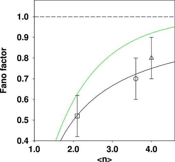
Comparison of reported Fano factors for vacuole populations, compared to two different theoretical expectations.
Three data points quoted in the SMOP paper are plotted: □ Haploid (glucose); ○ Diploid (glucose); ∆ Haploid (oleate). The solid black curve is the expectation from the shifted Poisson distribution (which is the incorrect distribution given the {fission; fusion} model) and the solid green curve is the expectation from the truncated Poisson distribution (which is the correct distribution given the model). The dashed line is for a Fano factor of 1. The solid curves were constructed by calculating a family of distributions and evaluating the mean and Fano factor.
Figure 3
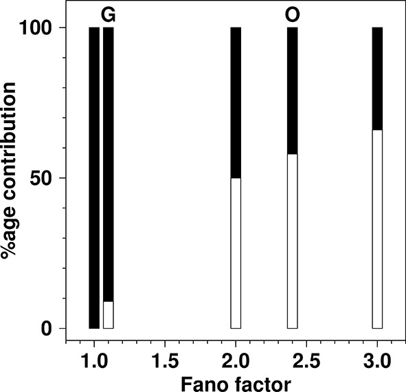
The percentage contribution to the total production rate from de novo production and from fission as a function of Fano factor in the {de novo, fission; decay} model.
For each value of the Fano factor shown, a bar is drawn to represent the total production rate. The filled part of the bar represents the contribution from de novo production inferred from the model and the open part of the bar represents the inferred rate from fission. Bars are shown for Fano factors of: 1.0 (100% de novo); 1.1 (experimentally observed for glucose growth (G) in SMOP paper; 9% de novo, 91% fission); 2.0 (boundary value, where de novo and fission contributions are equal); 2.4 (experimentally reported value for oleate growth (O) in SMOP paper; 42% de novo, 58% fission); 3.0 (value required for fission rate to be double the de novo rate). The total production rate from de novo processes is simply kde novo. The total rate from fission processes is kfission<n>. The relative proportions of the two processes were calculated using Equation 5.
Appendix 4 Figure 1
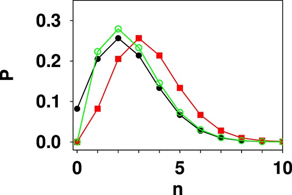
Comparison of Poisson (black filled circles), shifted Poisson (red filled squares), and truncated Poisson (green open circles) distributions calculated for λ = 2.5.
The values in a shifted Poisson distribution are the same as in the corresponding Poisson distribution, however the whole distribution is shifted to the right by one unit in n. The value at n = 0 is set to zero. In a truncated Poisson the value at n = 0 is set to zero, and the rest of the distribution has the same functional form as the corresponding Poisson distribution. Due to the loss of the n = 0 point then normalisation causes the remaining values to be slightly higher in the truncated Poisson distribution than in the corresponding Poisson distribution.
Tables
Table 1
Definition of terms in the SMOP model
| Process | Probability of process occurring in next δt in a particular cell containing n organelles1 | Process changes n by | Rate of process in sample of N cells2 |
|---|---|---|---|
| De novo | kde novoδt | 1 | kde novofnN |
| Fission | kfissionnδt | 1 | kfissionnfnN |
| Decay | γnδt | -1 | γnfnN |
| Fusion | kfusionn(n-1)δt | -1 | kfusionn(n-1)fnN |
-
1For example, if kfission = 0.02 then the probability of a cell with n = 2 organelles undergoing a fission event in the next 0.1 time units = 0.02x2x0.1 = 0.004.
-
2fn is the fraction of cells having n organelles. For example, if 23% of the cells have 2 organelles then f2 = 0.23. If, in a population of 1000 cells, f2 = 0.23 and kfission = 0.02 then the rate of cells changing from having n = 2 to n = 3 organelles at any one moment due to fission would be 0.02x2x0.23x1000 = 9.2 cells per time unit.
Additional files
-
Source code 1
Code for calculating time courses via simulation.
- https://doi.org/10.7554/eLife.10167.007
-
Source code 2
Code for calculating distributions via the recurrence relation.
- https://doi.org/10.7554/eLife.10167.008
Download links
A two-part list of links to download the article, or parts of the article, in various formats.
Downloads (link to download the article as PDF)
Open citations (links to open the citations from this article in various online reference manager services)
Cite this article (links to download the citations from this article in formats compatible with various reference manager tools)
Evaluation of predictions of the stochastic model of organelle production based on exact distributions
eLife 5:e10167.
https://doi.org/10.7554/eLife.10167


