A conformational fingerprint for amyloidogenic light chains
- Department of Bioscience, University of Milan, Italy
- Indian Institute of Science Education and Research Pune, India
- Institute of Molecular and Translational Cardiology, IRCCS, Policlinico San Donato, Italy
- Institute of Biological Chemistry, Academia Sinica, Taiwan
- Department of Pathophysiology and Transplantation, University of Milan, Italy
- Department of Molecular Medicine, University of Pavia, Italy
- Amyloidosis Research and Treatment Center, Fondazione IRCCS Policlinico San Matteo, Italy
- Institute of Biochemical Sciences, National Taiwan University, Taiwan
- International Institute for Sustainability with Knotted Chiral Meta Matter (SKCM2), Hiroshima University, Japan
Figures
Figure 1 with 3 supplements

Comparison of small-angle X-ray scattering (SAXS) data and single light-chain (LC) structures.
Kratky plots of for amyloidosis (AL) and multiple myeloma (MM) LCs. The experimental (orange) and theoretical (black) curves (top panels) and the associated residuals (bottom panels) indicate that AL-LC solution behavior deviates from reference structures more than MM-LC. SAXS was measured as follows: H3 measured in bulk (Hamburg), 3.4 mg/ml; H7 measured in bulk (Hamburg), 3.4 mg/ml; H18 measured by size-exclusion chromatography (SEC)-SAXS (ESRF [European Synchrotron radiation facility]) with the injection concentration of at 2.8 mg/ml; AL55 measured in bulk (ESRF), 2.6 mg/ml; M7 measured in bulk (Hamburg), 3.6 mg/ml; and M10 measured by SEC-SAXS with the injection concentration of 6.7 mg/ml (ESRF). Theoretical SAXS curves were calculated using crysol (Manalastas-Cantos et al., 2021). Log-log plots are shown in Figure 1—figure supplement 1.
Figure 1—figure supplement 1
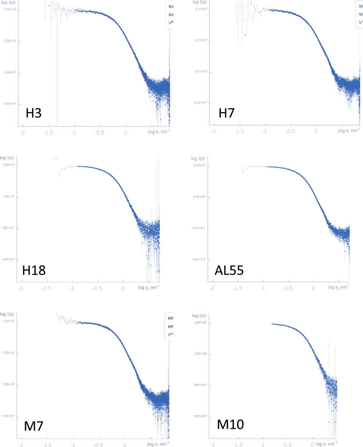
Log-log plots representing the small-angle X-ray scattering experimental curves for the six proteins.
Figure 1—figure supplement 2
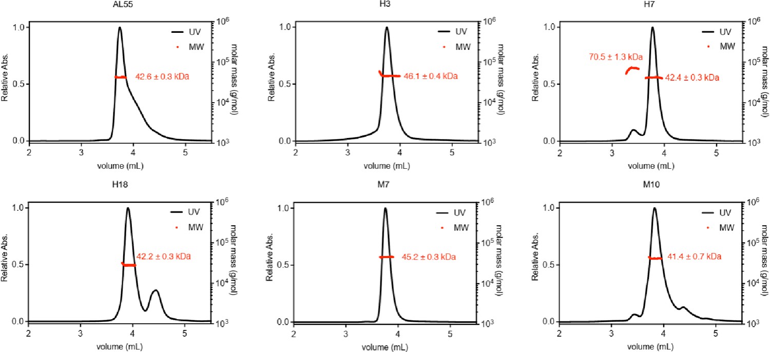
Size exclusion coupled multiangle light scattering analysis of purified light chains (AL55, H3, H7, H18, M7, and M10).
The name of each protein is labeled above their corresponding profile. The obtained molecular weight (MW) is highlighted in red.
Figure 1—figure supplement 3
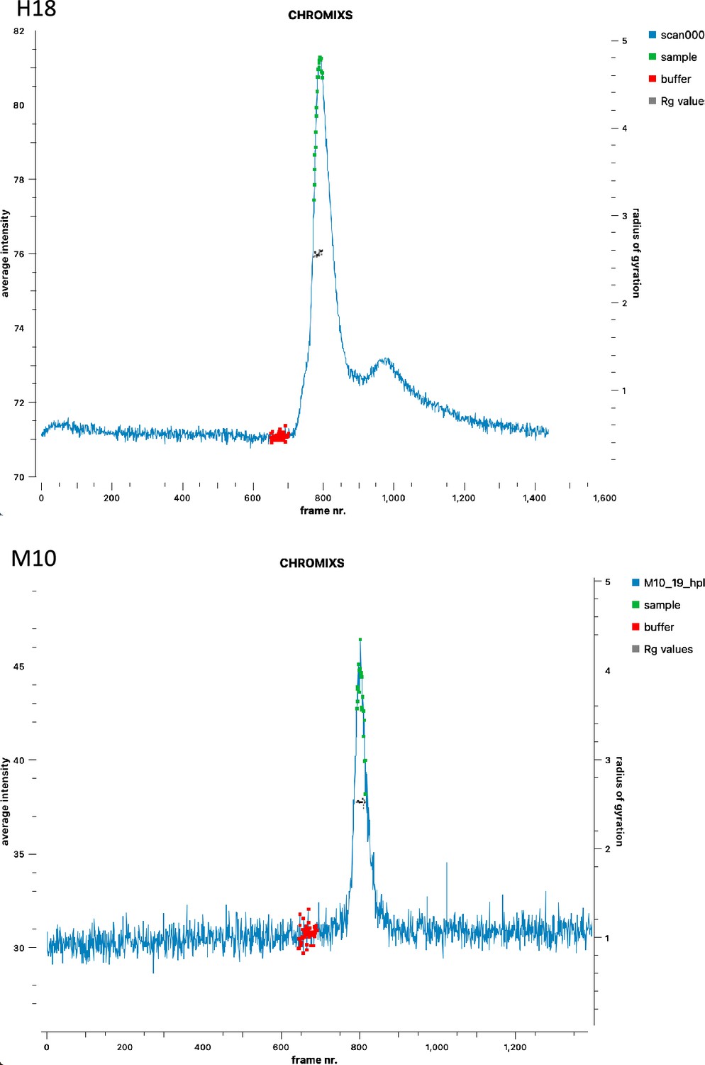
Small-angle X-ray scattering–size-exclusion chromatography average intensity for H18 and M10.
Selected frames for buffer and sample are reported together with the analysis of the estimated Rg values, indicating that the selection corresponds to homogeneous conformations.
Figure 2
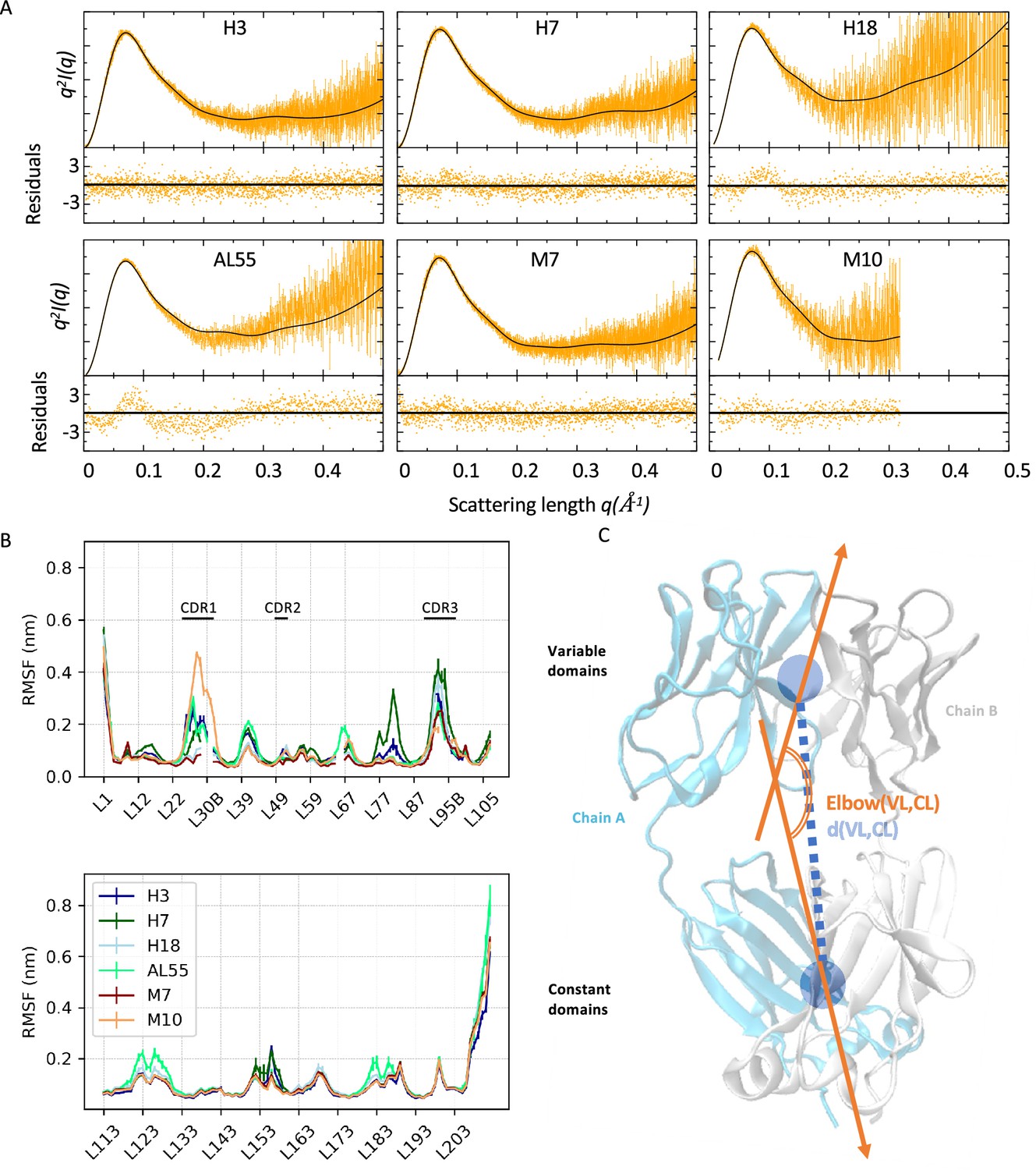
Light-chain small-angle X-ray scattering (SAXS)-driven molecular dynamics simulations.
(A) Kratky plots and associated residuals (bottom panels) comparing experimental (orange), and theoretical (black) curves obtained by averaging over the metainference ensemble for H3, H7, H18, AL55, M7, and M10, respectively. Theoretical SAXS curves were calculated using crysol (Manalastas-Cantos et al., 2021). (B) Residue-wise root mean square fluctuations (RMSFs) obtained by averaging the two metainference replicates and the two equivalent domains for the six systems studied. The top panel shows data for the variable domains, while the bottom panel shows data for the constant domain. Residues are reported using Chothia and Lesk numbering (Al-Lazikani et al., 1997). (C) Schematic representation of two global collective variables used to compare the conformational dynamics of the different systems, namely the distance between the center of mass of the variable domain (VL) and constant domain (CL) dimers and the angle describing the bending of the two domain dimers.
Figure 3

Free energy surfaces (FESs) for the six light-chain systems under study by metadynamics metainference molecular dynamics simulations.
For each system, the simulations are performed in duplicate. The x-axis represents the elbow angle, indicating the relative bending of the constant and variable domains (in radians), while the y-axis represents the distance in nm between the center of mass of the constant domain (CL) and variable domain (VL) dimers. The free energy is shown with color and isolines every 2kBT corresponding to 5.16 kJ/mol. On each FES are represented four regions (green, LB state; red, LS state; blue, H state; and black, G state), highlighting the main conformational states. For each region, a representative structure is reported in a rectangle of the same color.
Figure 4 with 6 supplements
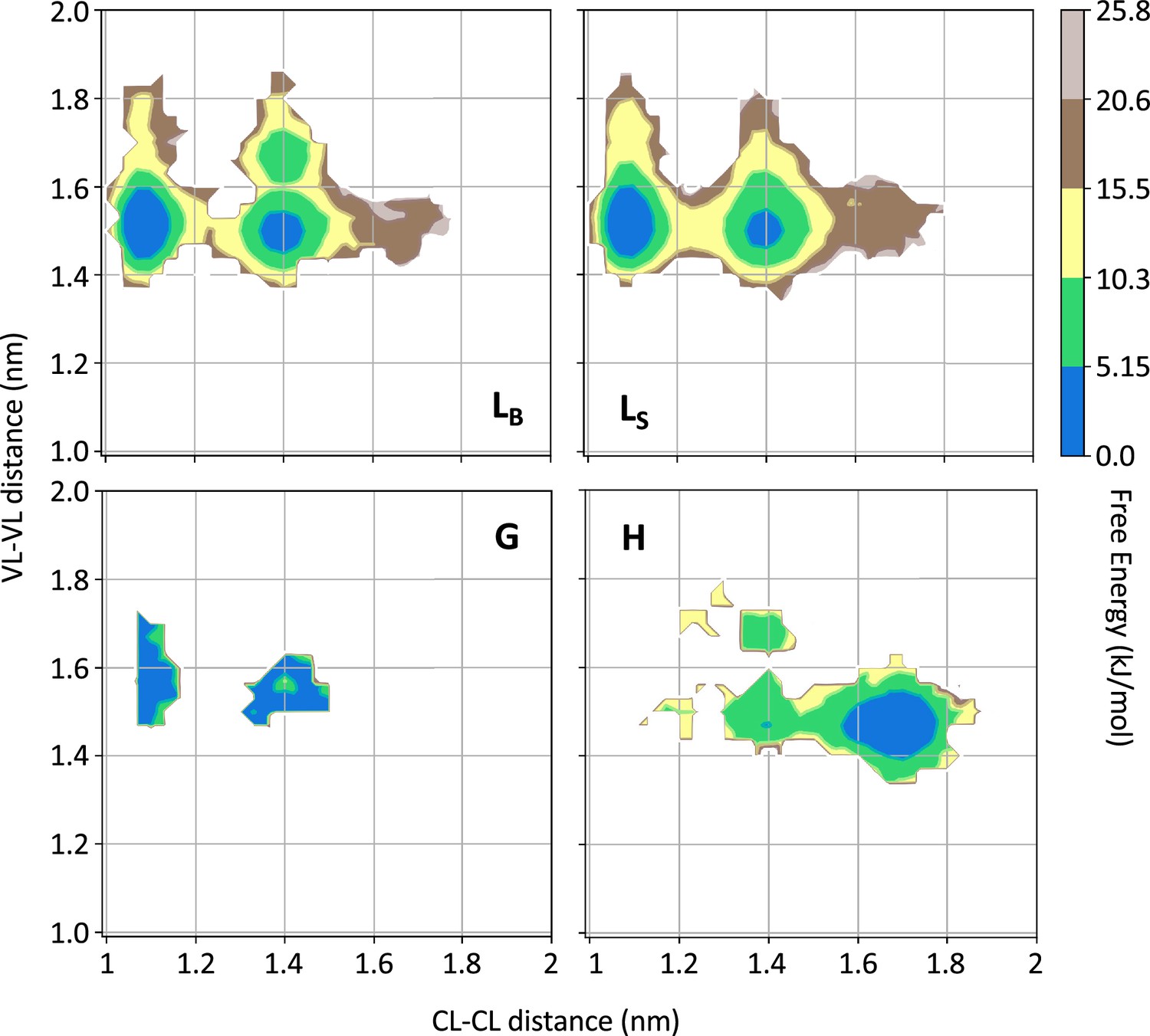
Free energy surfaces for the four substates identified in Figure 3 in the case of the first H3 metainference simulation.
The x-axis shows the distance between the centers of mass of the constant domains, while the y-axis shows the distance between the centers of mass of the variable domains. The free energy is shown with color and isolines every 2kBT corresponding to 5.16 kJ/mol. See also Figure 4—figure supplements 1–6 for the same analysis on the other simulations.
Figure 4—figure supplement 1

Free energy surfaces for the four substates identified in Figure 3 in the case of the second H3 metainference simulation.
The x-axis shows the distance between the centers of mass of the constant domains, while the y-axis shows the distance between the centers of mass of the variable domains. The free energy is shown with color and isolines every 2kBT corresponding to 5.16 kJ/mol.
Figure 4—figure supplement 2
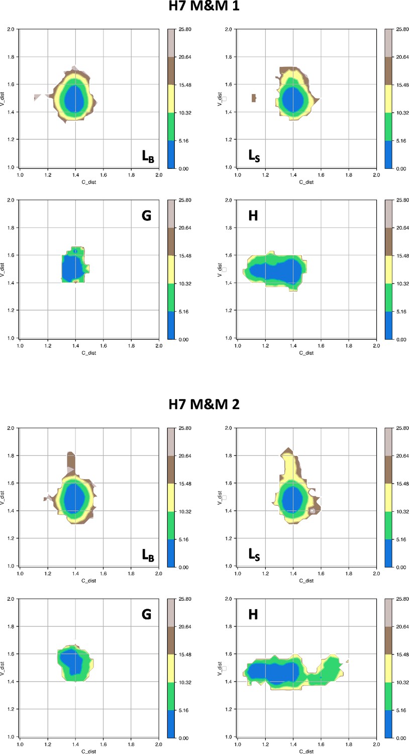
Free energy surfaces for the four substates identified in Figure 3 in the case of the first (top) and second (bottom) H7 metainference simulation.
The x-axis shows the distance between the centers of mass of the constant domains, while the y-axis shows the distance between the centers of mass of the variable domains. The free energy is shown with color and isolines every 2kBT corresponding to 5.16 kJ/mol.
Figure 4—figure supplement 3
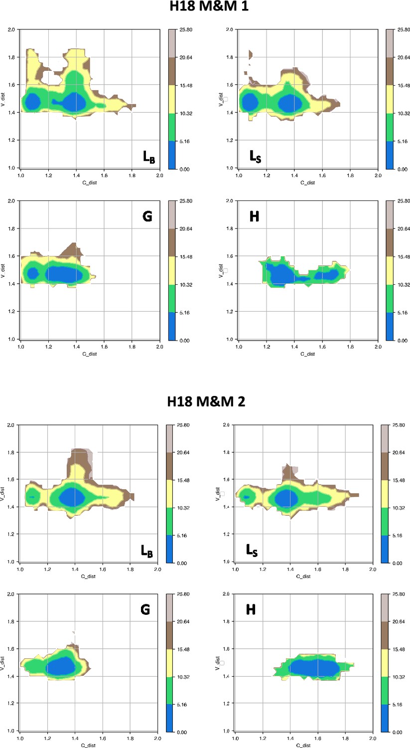
Free energy surfaces for the four substates identified in Figure 3 in the case of the first (top) and second (bottom) H18 metainference simulation.
The x-axis shows the distance between the centers of mass of the constant domains, while the y-axis shows the distance between the centers of mass of the variable domains. The free energy is shown with color and isolines every 2kBT corresponding to 5.16 kJ/mol.
Figure 4—figure supplement 4
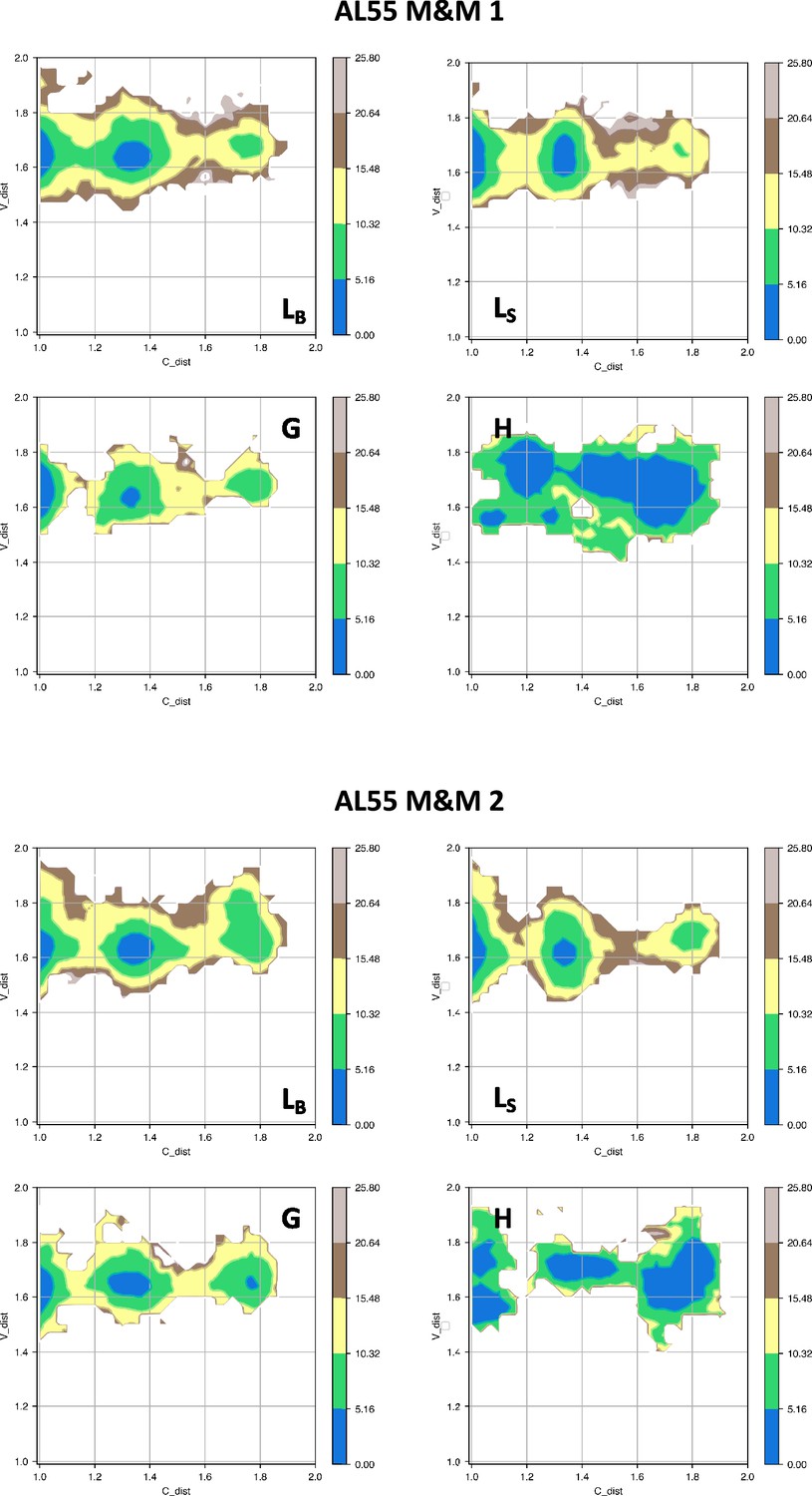
Free energy surfaces for the four substates identified in Figure 3 in the case of the first (top) and second (bottom) AL55 metainference simulation.
The x-axis shows the distance between the centers of mass of the constant domains, while the y-axis shows the distance between the centers of mass of the variable domains. The free energy is shown with color and isolines every 2kBT corresponding to 5.16 kJ/mol.
Figure 4—figure supplement 5
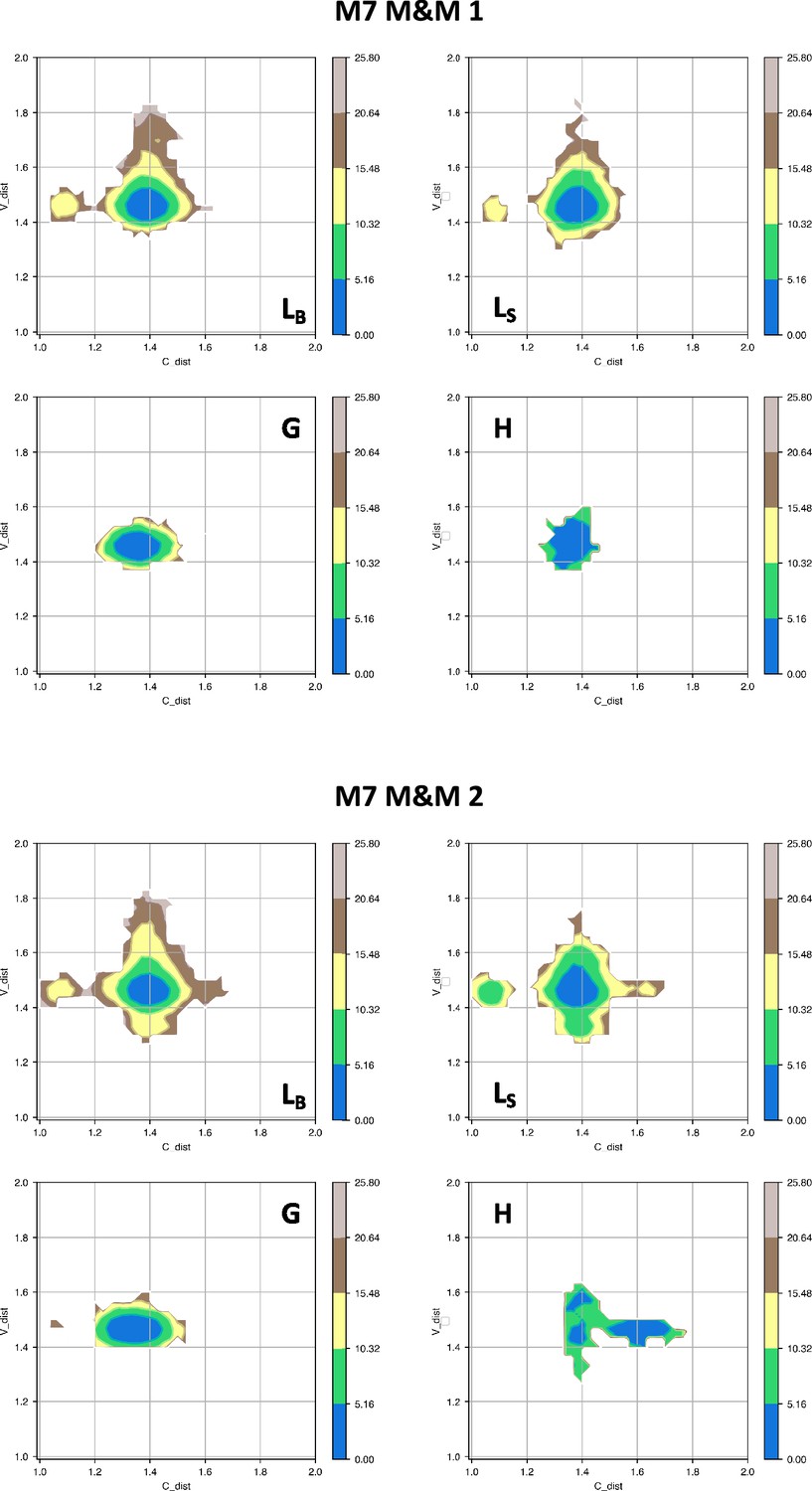
Free energy surfaces for the four substates identified in Figure 3 in the case of the first (top) and second (bottom) M7 metainference simulation.
The x-axis shows the distance between the centers of mass of the constant domains, while the y-axis shows the distance between the centers of mass of the variable domains. The free energy is shown with color and isolines every 2kBT corresponding to 5.16 kJ/mol.
Figure 4—figure supplement 6
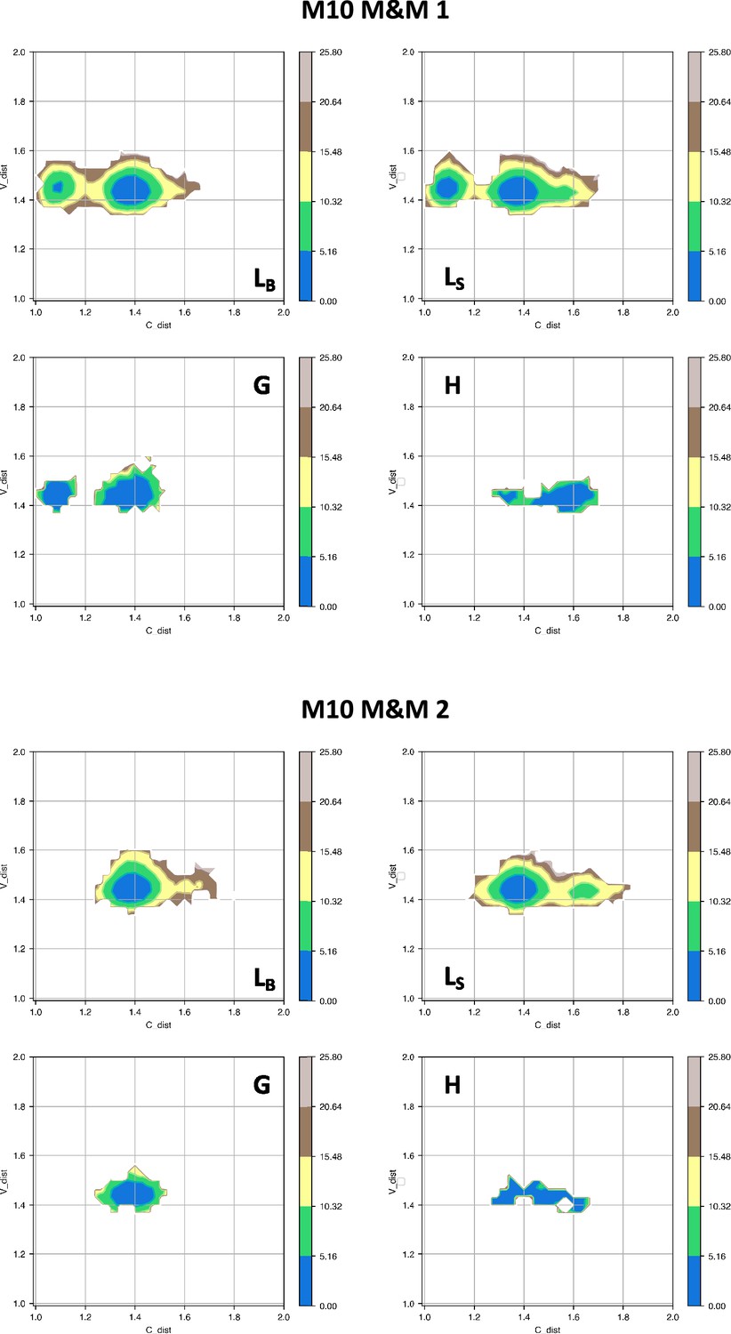
Free energy surfaces for the four substates identified in Figure 3 in the case of the first (top) and second (bottom) M10 metainference simulation.
The x-axis shows the distance between the centers of mass of the constant domains, while the y-axis shows the distance between the centers of mass of the variable domains. The free energy is shown with color and isolines every 2kBT corresponding to 5.16 kJ/mol.
Figure 5 with 10 supplements
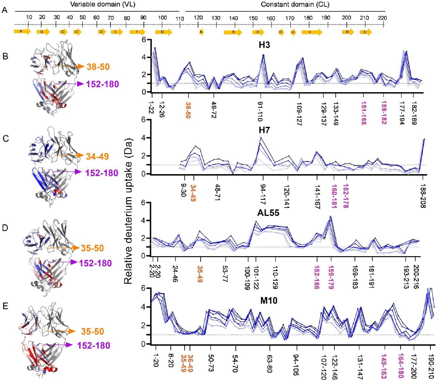
Hydrogen-deuterium exchange mass spectrometry analysis.
(A) The top panel represents the simplified presentation of the primary structure of a light chain, including variable domain (VL) and constant domain (CL). The location of β-strands according to Chothia and Lesk (Al-Lazikani et al., 1997). (B) The structural mapping and butterfly plot of relative deuterium uptake (Da) of H3. Chain A of H3 structure is colored in a gradient of blue–white–red for an uptake of 0–30% at an exchange time of 30 min. Chain B is shown in gray (right-hand panel). The butterfly plot showing relative deuterium uptake at all time points from 0.5 to 240 min on a gradient of light to dark blue (left-hand panel). (C–E) are the figures corresponding to H7, AL55, and M10, respectively, with the same color coding as in (B). The overall sequence coverage for all proteins was >90%, with a redundancy of >4.0. The VL-VL domains interface peptides covering amino acid residues 34–50 are labeled in orange, while the CL-CL interface region containing 152–180 amino acids is labeled in magenta. Collectively, they form VL-CL interface, which is important to define the H state.
Figure 5—figure supplement 1
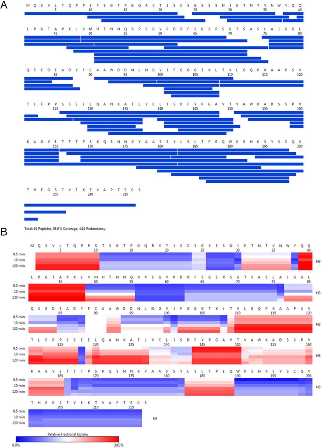
H3 HDX coverage and uptake.
(A) Peptide coverage map of protein H3. The total number of peptides is 61, with a coverage of 98.6% and a redundancy of 4.16. (B) As shown on the left, heat map as a function of hydrogen-deuterium exchange-time at different time points. The relative deuterium uptake is color-coded from blue-to-white-to-red for 0–30% as indicated by the scale bar below.
Figure 5—figure supplement 2
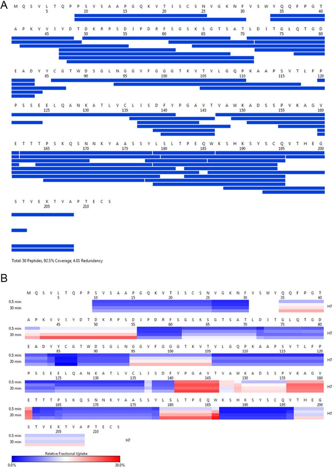
H7 HDX coverage and uptake.
(A) Peptide coverage map of protein H7. The total number of peptides is 50, with a coverage of 92.5% and a redundancy of 4.01. (B) Heat map as a function of hydrogen-deuterium exchange-time at different time points as shown on the left. The relative deuterium uptake is color-coded from blue-to-white-to-red for 0–30% as shown by the scale bar below.
Figure 5—figure supplement 3
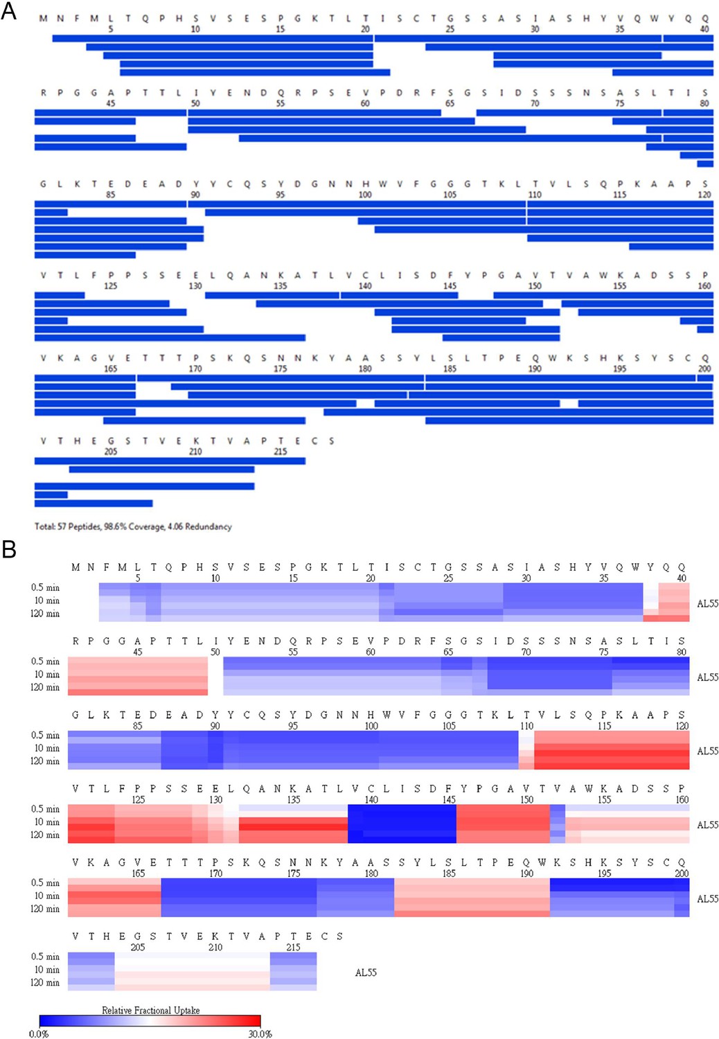
AL55 HDX coverage and uptake.
(A) Peptide coverage map of protein AL55. The total number of peptides is 57, with a coverage of 98.6% and a redundancy of 4.06. (B) Heat map as a function of hydrogen-deuterium exchange-time at different time points as shown on the left. The relative deuterium uptake is color-coded from blue-to-white-to-red for 0–30% as shown by the scale bar below.
Figure 5—figure supplement 4

M10 HDX coverage and uptake.
(A) Peptide coverage map of protein M10. The total number of peptides is 62, with a coverage of 99.1% and a redundancy of 4.69. (B) As shown on the left, heat map as a function of hydrogen-deuterium exchange-time at different time points. The relative deuterium uptake is color-coded from blue-to-white-to-red for 0–30% as indicated by the scale bar below.
Figure 5—figure supplement 5
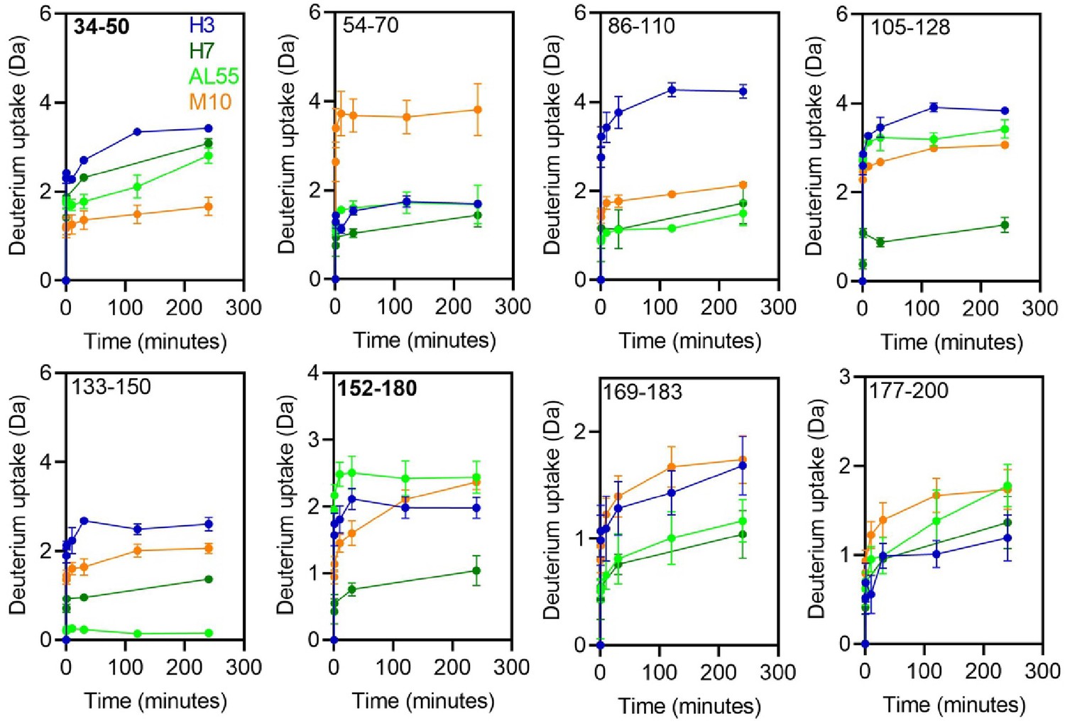
Hydrogen-deuterium exchange kinetics of deuterium uptake at each time points from 0 to 240 min for the selected peptides.
The colors corresponding to each protein H3 (blue), H7 (green), AL55 (light green), and M10 (orange) are shown in the first panel. The residue numbers corresponding to the individual peptides are shown in the upper-left corner of the individual panels. The panels for peptides containing residues 34–50 and 152–180 highlighted in bold are of our interest in this study.
Figure 5—figure supplement 6
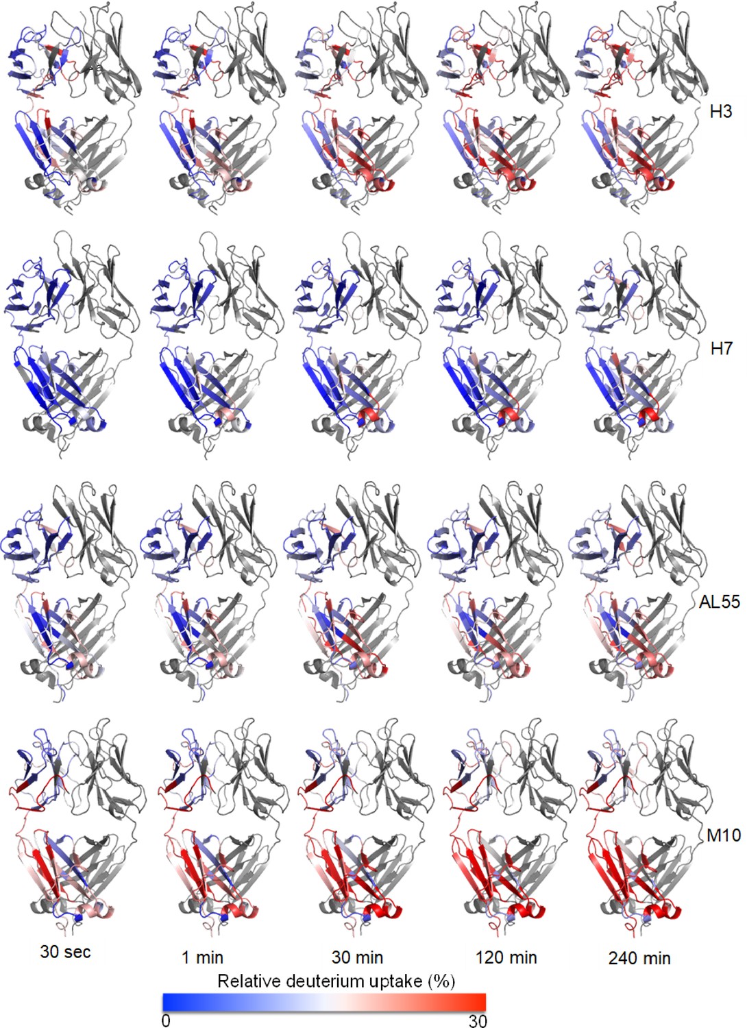
Structural mapping of relative deuterium uptake on chain A of each dimeric light chain: relative deuterium uptake of H3, H7, AL55, and M10 at different time points of 0.5–240 min on a scale of 0–30% uptake.
The color gradient is from blue–white–red. Blue means no exchange, and red means an exchange of 30%. The protein name is written on the right-hand side of each panel. Chain B is colored in gray.
Figure 5—video 1
3D structure of H3, color-coded by hydrogen-deuterium exchange and rotating 360°.
Figure 5—video 2
3D structure of H7, color-coded by hydrogen-deuterium exchange and rotating 360°.
Figure 5—video 3
3D structure of AL55, color-coded by hydrogen-deuterium exchange and rotating 360°.
Figure 5—video 4
3D structure of M10, color-coded by hydrogen-deuterium exchange and rotating 360°.
Figure 6 with 7 supplements
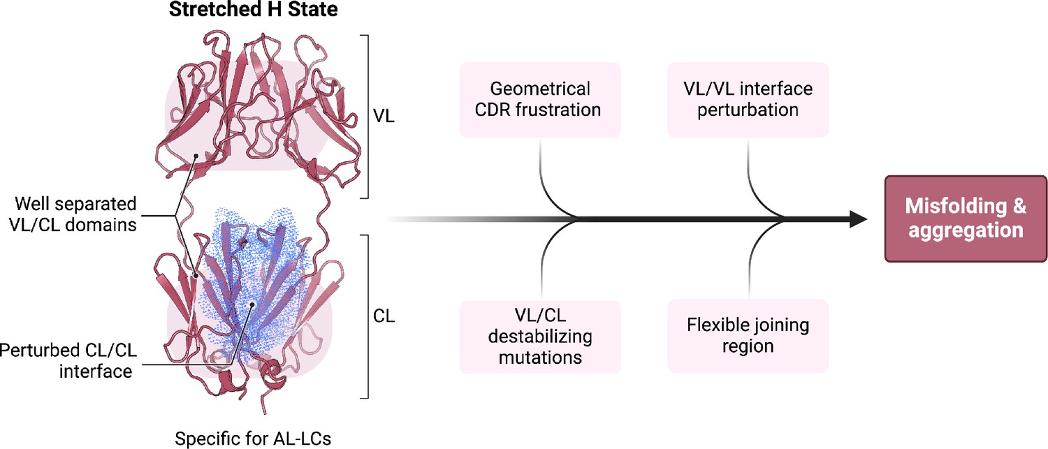
Schematic representation summarizing our findings in the context of previous work on the biophysical properties of amyloidogenic light chains (LCs).
We propose that the H state is the conformational fingerprint distinguishing amyloidosis (AL) LCs from other LCs, which, together with other features, contributes to the amyloidogenicity of AL LCs.
Figure 6—figure supplement 1

Zoom-in on the crystal structure of M7 to show the hydrophobic contact between A40 in the variable domain (VL) and T165 in the constant domain (CL).
The multiple sequence alignment for M7, H18, and their germline sequence (IGLV3-19*01 for the VL and IGLC2*02 for the CL) is reported below.
Figure 6—figure supplement 2
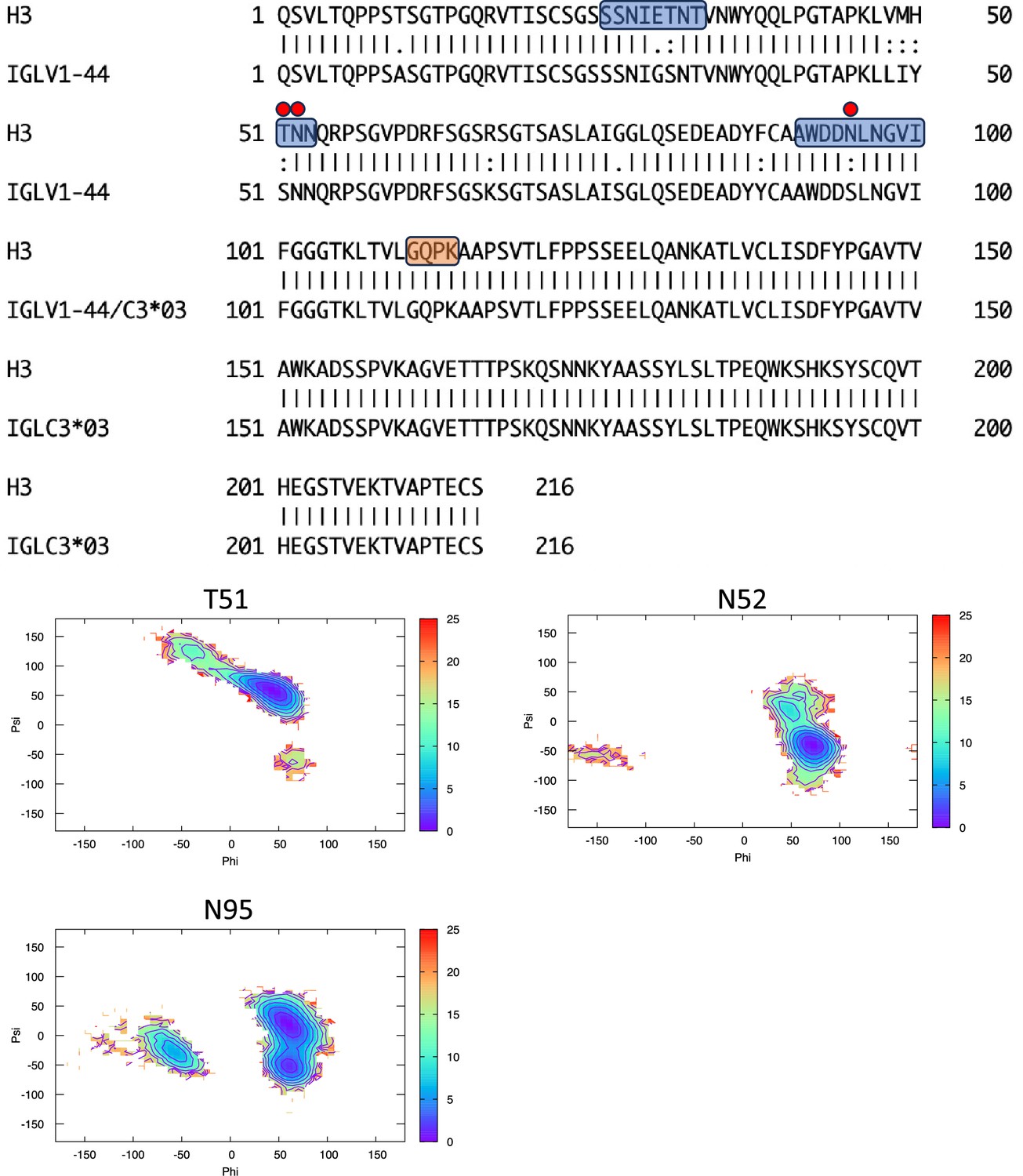
Pairwise sequence alignment between H3 and its corresponding germline as identified by igBLAST using the IGMT databases.
The three complementarity-determining regions and the linker region are highlighted in light blue and orange, respectively. The red circles indicate residues for which the left alpha is the most populated region in the Ramachandran plot. Free energy surfaces (in kJ/mol) representing the Ramachandran plot for the indicated residues are reported in the bottom panels.
Figure 6—figure supplement 3
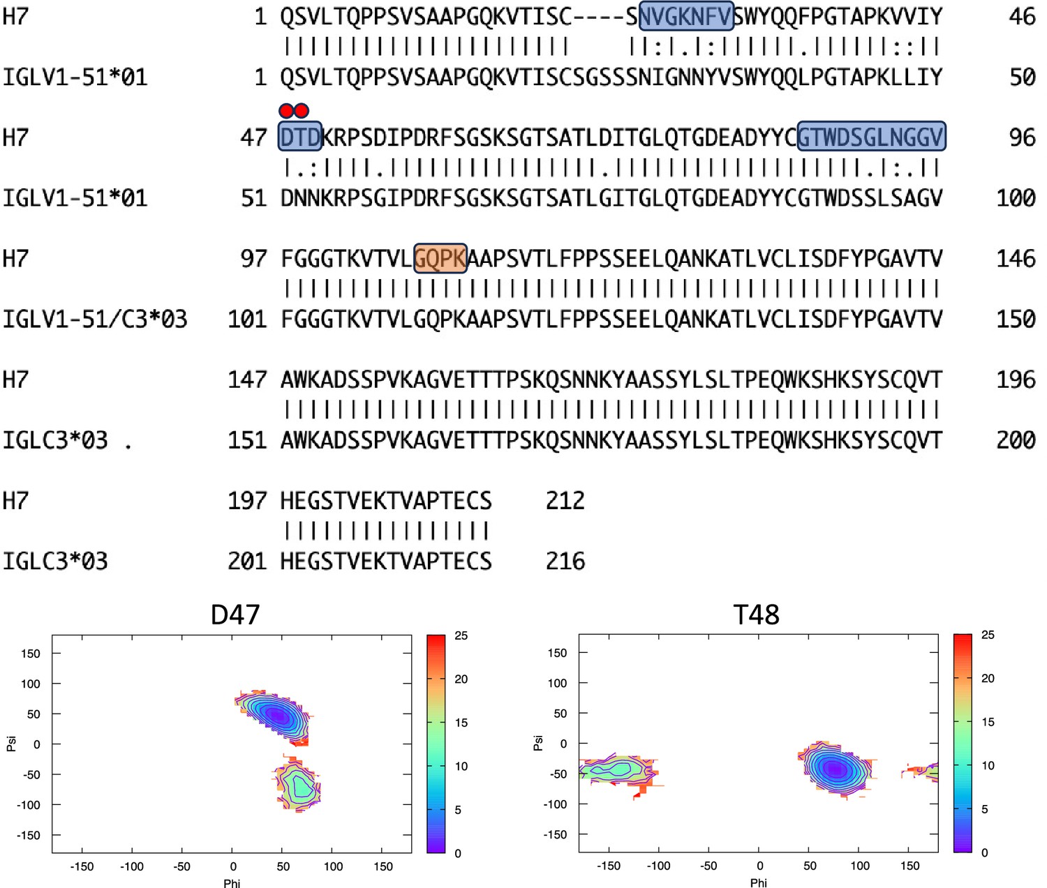
Pairwise sequence alignment between H7 and its corresponding germline as identified by igBLAST using the IGMT databases.
The three complementarity-determining regions and the linker region are highlighted in light blue and orange, respectively. The red circles indicate residues for which the left alpha is the most populated region in the Ramachandran plot. Free energy surfaces (in kJ/mol) representing the Ramachandran plot for the indicated residues are reported in the bottom panels.
Figure 6—figure supplement 4
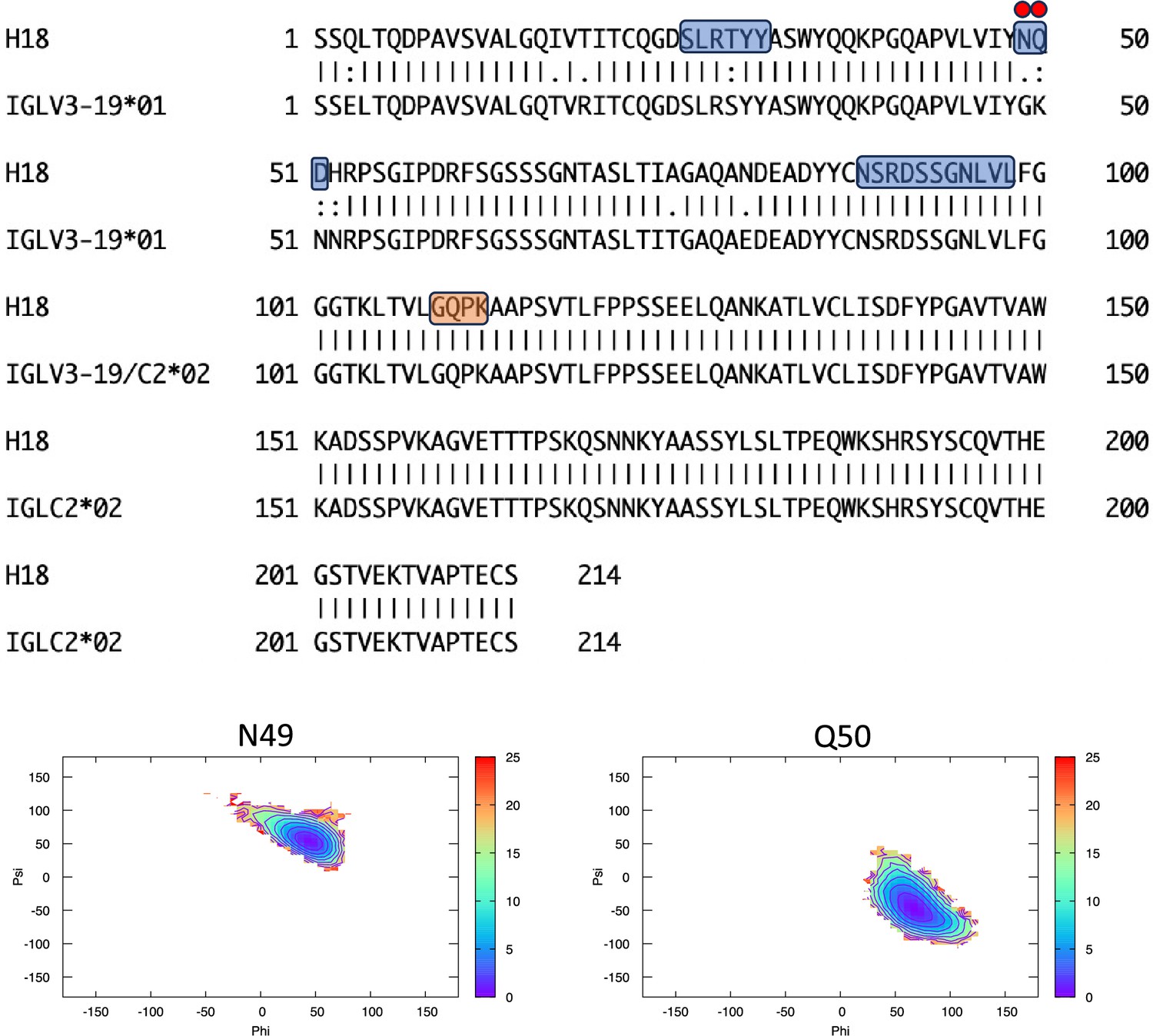
Pairwise sequence alignment between H18 and its corresponding germline as identified by igBLAST using the IGMT databases.
The three complementarity-determining regions and the linker region are highlighted in light blue and orange, respectively. The red circles indicate residues for which the left alpha is the most populated region in the Ramachandran plot. Free energy surfaces (in kJ/mol) representing the Ramachandran plot for the indicated residues are reported in the bottom panels.
Figure 6—figure supplement 5
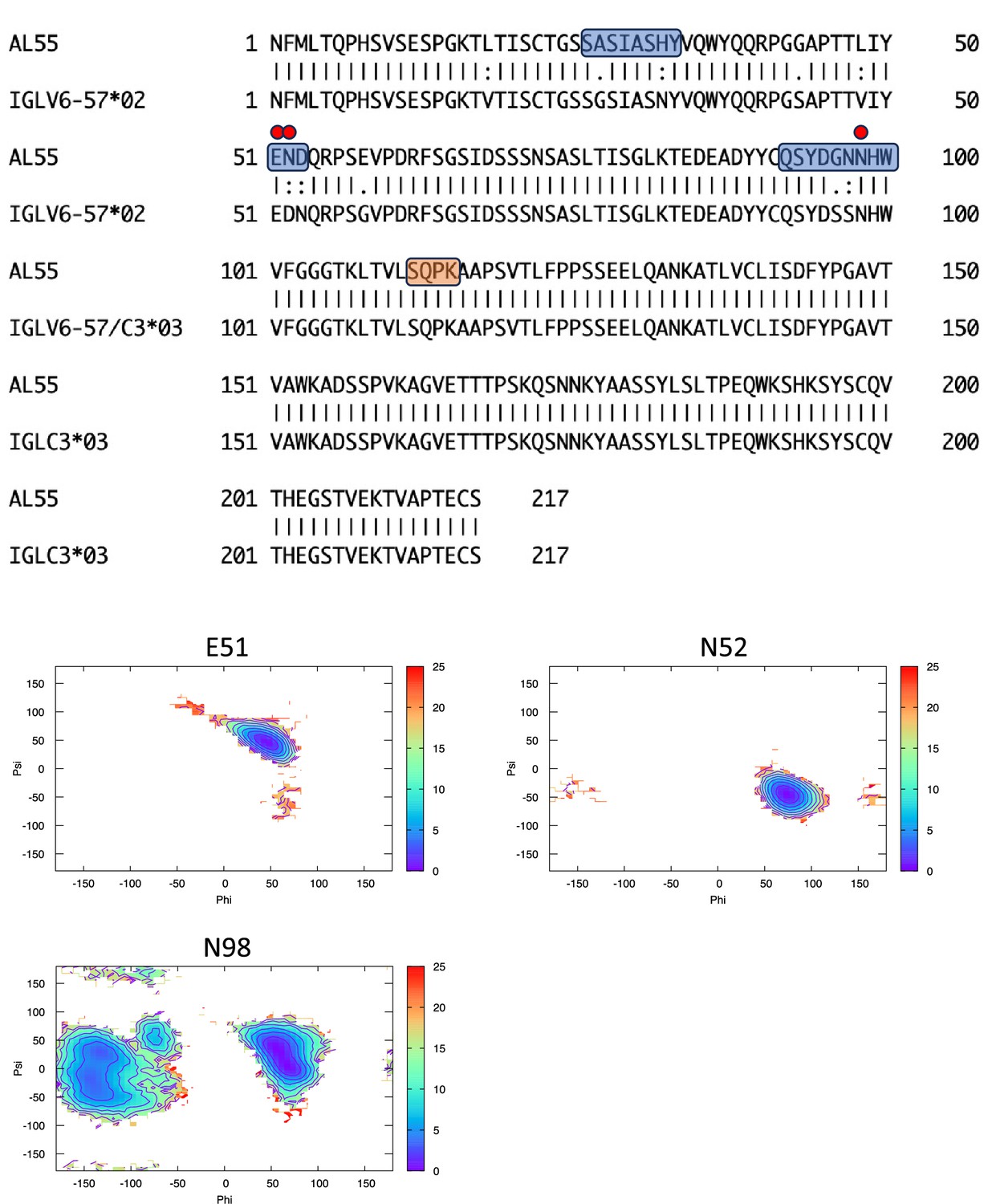
Pairwise sequence alignment between AL55 and its corresponding germline as identified by igBLAST using the IGMT databases.
The three complementarity-determining regions and the linker region are highlighted in light blue and orange, respectively. The red circles indicate residues for which the left alpha is the most populated region in the Ramachandran plot. Free energy surfaces (in kJ/mol) representing the Ramachandran plot for the indicated residues are reported in the bottom panels.
Figure 6—figure supplement 6
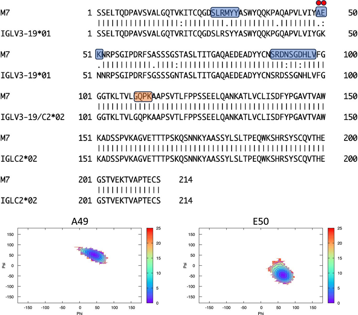
Pairwise sequence alignment between M7 and its corresponding germline as identified by igBLAST using the IGMT databases.
The three complementarity-determining regions and the linker region are highlighted in light blue and orange, respectively. The red circles indicate residues for which the left alpha is the most populated region in the Ramachandran plot. Free energy surfaces (in kJ/mol) representing the Ramachandran plot for the indicated residues are reported in the bottom panels.
Figure 6—figure supplement 7
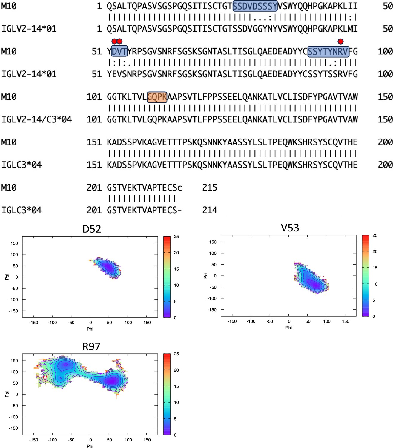
Pairwise sequence alignment between M10 and its corresponding germline as identified by igBLAST using the IGMT databases.
The three complementarity-determining regions and the linker region are highlighted in light blue and orange, respectively. The red circles indicate residues for which the left alpha is the most populated region in the Ramachandran plot. Free energy surfaces (in kJ/mol) representing the Ramachandran plot for the indicated residues are reported in the bottom panels.
Tables
Table 1
LC systems studied in this work.
The table includes information about the germline, phenotype, method to obtain structure, the SAXS curves, and the radius of gyration derived from the SAXS data for all the model proteins studied in this work.
| LC | Germline | Phenotype | Structure | SAXS χ2 q < 0.5 Å (q < 0.3) | Rg (SAXS) (nm) |
|---|---|---|---|---|---|
| H3 | IGLV1-44*01 | AL | 5MTL | 1.6 (1.9) | 2.57 ± 0.02 |
| H7 | IGLV1-51*01 | AL | 5MUH | 2.8 (4.0) | 2.56 ± 0.02 |
| H18 | IGLV3-19*01 | AL | Homology | 1.6 (1.9) | 2.56 ± 0.01 |
| AL55 | IGLV6-57*02 | AL | Homology | 5.1 (7.8) | 2.58 ± 0.04 |
| M7 | IGLV3-19*01 | MM | 5MVG | 1.2 (1.2) | 2.50 ± 0.02 |
| M10 | IGLV2-14*03 | MM | AF2 | 1.2 (1.2) | 2.51 ± 0.01 |
-
AL, amyloidosis; LC, light chain; MM, multiple myeloma; SAXS, small-angle X-ray scattering.
Table 2
Metainference simulations performed in this work for the six systems.
For each metainference simulation, the simulation time per replica with the number of replicas is reported; the χ2 of the resulting conformational ensemble with the experimental SAXS curve, the range q < 0.3 Å is the one used as restraint in the simulation; the average radius of gyration with error estimated by block averaging.
| LC code | Simulation | Length per replica (ns) (# replicas) | SAXS χ2 q < 0.5 Å (q < 0.3) | Average Rg (nm) |
|---|---|---|---|---|
| H3 | M&M 1 | 1530 (60) | 1.2 (1.1) | 2.56 ± 0.02 |
| M&M 2 | 1520 (60) | 1.2 (1.1) | 2.56 ± 0.02 | |
| H7 | M&M 1 | 1627 (60) | 1.1 (1.2) | 2.54 ± 0.04 |
| M&M 2 | 1545 (60) | 1.1 (1.2) | 2.54 ± 0.05 | |
| H18 | M&M 1 | 1643 (60) | 1.4 (1.6) | 2.53 ± 0.03 |
| M&M 2 | 1529 (60) | 1.4 (1.7) | 2.54 ± 0.03 | |
| AL55 | M&M 1 | 1545 (60) | 2.7 (3.0) | 2.59 ± 0.02 |
| M&M 2 | 1591 (60) | 2.5 (2.7) | 2.58 ± 0.05 | |
| M7 | M&M 1 | 1623 (60) | 1.2 (1.2) | 2.52 ± 0.03 |
| M&M 2 | 1530 (60) | 1.1 (1.2) | 2.52 ± 0.03 | |
| M10 | M&M 1 | 987 (60) | 1.1 (1.1) | 2.53 ± 0.07 |
| M&M 2 | 995 (60) | 1.1 (1.1) | 2.54 ± 0.05 |
-
LC, light chain; M&M, metadynamics metainference; SAXS, small-angle X-ray scattering.
Table 3
Populations of the four states shown in Figure 3 resulting from the two independent metadynamics metainference simulations performed for each of the six LCs.
The population of the H state, which is supposed to be a fingerprint specific for AL-LCs, is in bold.
| % | H3 | H7 | H18 | AL55 | M7 | M10 |
|---|---|---|---|---|---|---|
| LB | 62.0 ± 0.4 | 72.3 ± 2.5 | 22.9 ± 2.8 | 48.3 ± 0.1 | 46.8 ± 0.1 | 48.4 ± 0.3 |
| LS | 33.0 ± 0.2 | 15.2 ± 2.7 | 38.4 ± 2.1 | 32.5 ± 2.0 | 35.0 ± 0.1 | 49.1 ± 1.5 |
| G | 0.2 ± 0.1 | 0.8 ± 0.4 | 33.8 ± 3.8 | 10.5 ± 1.4 | 17.6 ± 0.1 | 1.8 ± 0.6 |
| H | 4.8 ± 0.5 | 11.7 ± 0.5 | 5.0 ± 1.0 | 8.7 ± 0.5 | 0.6 ± 0.2 | 0.8 ± 0.6 |
-
AL, amyloidosis; LC, light chain.
Key resources table
| Reagent type (species) or resource | Designation | Source or reference | Identifiers | Additional information |
|---|---|---|---|---|
| Strain, strain background (Escherichia coli) | DH5α | NEB 5-alpha | Cat# C2987H | Chemical competent cells |
| Strain, strain background (E. coli) | BL21(DE3) | NEB | Cat# C2527H | Chemical competent cells |
| Peptide, recombinant protein | H3 | Oberti et al., 2017 | NA | |
| Peptide, recombinant protein | H7 | Oberti et al., 2017 | NA | |
| Peptide, recombinant protein | AL55 | Puri et al., 2025 | NA | |
| Peptide, recombinant protein | H18 | Oberti et al., 2017 | NA | |
| Peptide, recombinant protein | M7 | Oberti et al., 2017 | NA | |
| Peptide, recombinant protein | M10 | Oberti et al., 2017 | NA | |
| Recombinant DNA reagent (plasmid) | pET21b(+)-H3 | Oberti et al., 2017 | NA | |
| Recombinant DNA reagent (plasmid) | pET21b(+)-H7 | Oberti et al., 2017 | NA | |
| Recombinant DNA reagent (plasmid) | pET21b(+)-AL55 | Puri et al., 2025 | NA | |
| Recombinant DNA reagent (plasmid) | pET21b(+)-H18 | Oberti et al., 2017 | NA | |
| Recombinant DNA reagent (plasmid) | pET21b(+)-M7 | Oberti et al., 2017 | NA | |
| Recombinant DNA reagent (plasmid) | pET21b(+)-M10 | Oberti et al., 2017 | NA | |
| Software, algorithm | PLGS | Waters | RRID:SCR_016664 | Section ‘Hydrogen-deuterium mass exchange spectrometry’ http://www.waters.com/ |
| Software, algorithm | DynamX | Waters | Section ‘Hydrogen-deuterium mass exchange spectrometry’ http://www.waters.com/ | |
| Software, algorithm | PyMOL | Schrodinger LLC | RRID:SCR_000305 | Section ‘Hydrogen-deuterium mass exchange spectrometry’ http://www.pymol.org/ |
| Software, algorithm | GraphPad Prism | GraphPad | RRID:SCR_002798 | Section ‘Hydrogen-deuterium mass exchange spectrometry’ http://www.graphpad.com/ |
| Software, algorithm | ATSAS 3 package | Manalastas-Cantos et al., 2021 | RRID:SCR_015648 | Section ‘Small-angle X-ray scattering’ http://www.embl-hamburg.de/biosaxs/atsas-online/ |
| Software, algorithm | GROMACS 2019 | Abraham et al., 2015 | RRID:SCR_014565 | Section ‘Molecular dynamics simulations’ https://www.gromacs.org/ |
| Software, algorithm | PLUMED2 v2.9 | Tribello et al., 2014 | RRID:SCR_021952 | Section ‘Molecular dynamics simulations’ https://www.plumed.org/ |
| Other | Hi prep QFF- 20 ml column | Cytiva | Product code 28936543 | Section ‘Protein production and purification’ |
| Other | Superdex 200 10/300 increase | Cytiva | Cat# 28990946 | Section ‘Protein production and purification’ |
| Other | Superdex 75 10/300 GL | Cytiva | Cat# 17517401 | Section ‘Protein production and purification’ |
| Other | Immobilized pepsin digestion column | Waters | (Waters Enzymate BEH Pepsin, 2.1 × 30 mm) | Section ‘Hydrogen-deuterium mass exchange spectrometry’ |
| Other | Isopropyl-β-d-thiogalactopyranoside (IPTG) | Himedia | RM2578 | Section ‘Protein production and purification’ |
| Other | Guanidinium chloride | Sigma-Aldrich | G3272-10KG | Section ‘Protein production and purification’ |
| Other | D2O | Sigma-Aldrich | CAS 7789-20-0 | Section ‘Hydrogen-deuterium mass exchange spectrometry’ |
Additional files
-
Supplementary file 1
Supplementary tables.
(a) Pairwise sequence identity (above diagonal) and similarity (below diagonal) for the six systems under study. On the diagonal is reported the germline identified by igBLAST using the IGMT database. (b) HDX-MS data summary.
- https://cdn.elifesciences.org/articles/102002/elife-102002-supp1-v1.docx
-
MDAR checklist
- https://cdn.elifesciences.org/articles/102002/elife-102002-mdarchecklist1-v1.docx
Download links
A two-part list of links to download the article, or parts of the article, in various formats.
Downloads (link to download the article as PDF)
Open citations (links to open the citations from this article in various online reference manager services)
Cite this article (links to download the citations from this article in formats compatible with various reference manager tools)
A conformational fingerprint for amyloidogenic light chains
eLife 13:RP102002.
https://doi.org/10.7554/eLife.102002.3


