A versatile pipeline for the multi-scale digital reconstruction and quantitative analysis of 3D tissue architecture
- Max Planck Institute of Molecular Cell Biology and Genetics, Germany
- Rohto Pharmaceutical, Japan
- Moscow State University, Russia
Figures
Figure 1 with 5 supplements
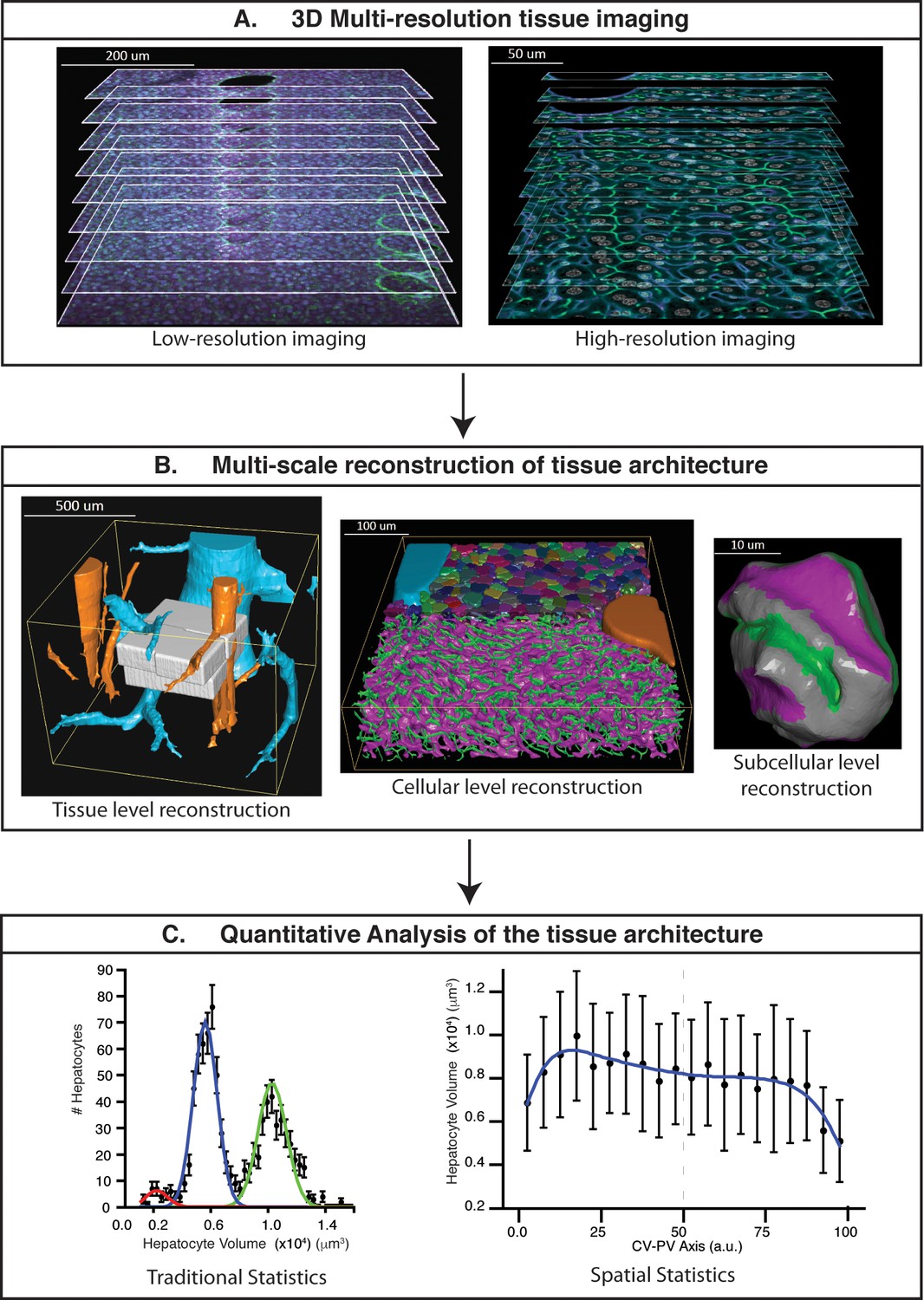
Schematic representation of the proposed pipeline.
(A) 3D multi-resolution image acquisition: example of arrays of 2D images of liver tissue acquired at different resolutions. Low- (1 μm × 1 μm × 1 μm per voxel) and high- (0.3 μm × 0.3 μm × 0.3 μm per voxel) resolution images on the left and right sides, respectively. (B) Multi-scale reconstruction of tissue architecture: on the left, reconstruction of a liver lobule showing tissue-level information, i.e., the localization and relative orientation of key structures such as the portal vein (PV) (orange) and central vein (CV) (light blue). The high-resolution images registered into the low-resolution one are shown in white. On the middle, a cellular-level reconstruction of liver showing the main components forming the tissue, i.e., bile canalicular (BC) network (green), sinusoidal network (magenta) and cells (random colours). The reconstruction corresponds to one of the high-resolution cubes (white) registered on the liver lobule reconstruction (left side). On the right, reconstruction of a single hepatocyte showing subcellular-level information, i.e., apical (green), basal (magenta) and lateral (grey) contacts. (C) Quantitative analysis of the tissue architecture: example of the statistical analysis performed over a morphometric tissue parameter (hepatocyte volume) using the information extracted from the multi-scale reconstruction. On the left, hepatocyte volume distribution over the sample (traditional statistics). On the right, spatial variability (spatial statistics) of the same parameter within the liver lobule. Our workflow allows not only to perform traditional statistical analysis of different morphometric parameters but also to perform spatial characterizations of them. The graphs were generated from the analysis of one high-resolution cube of the multi-scale reconstruction (the one shown in middle of panel B). Boundary cells were excluded from the analysis.
Figure 1—figure supplement 1
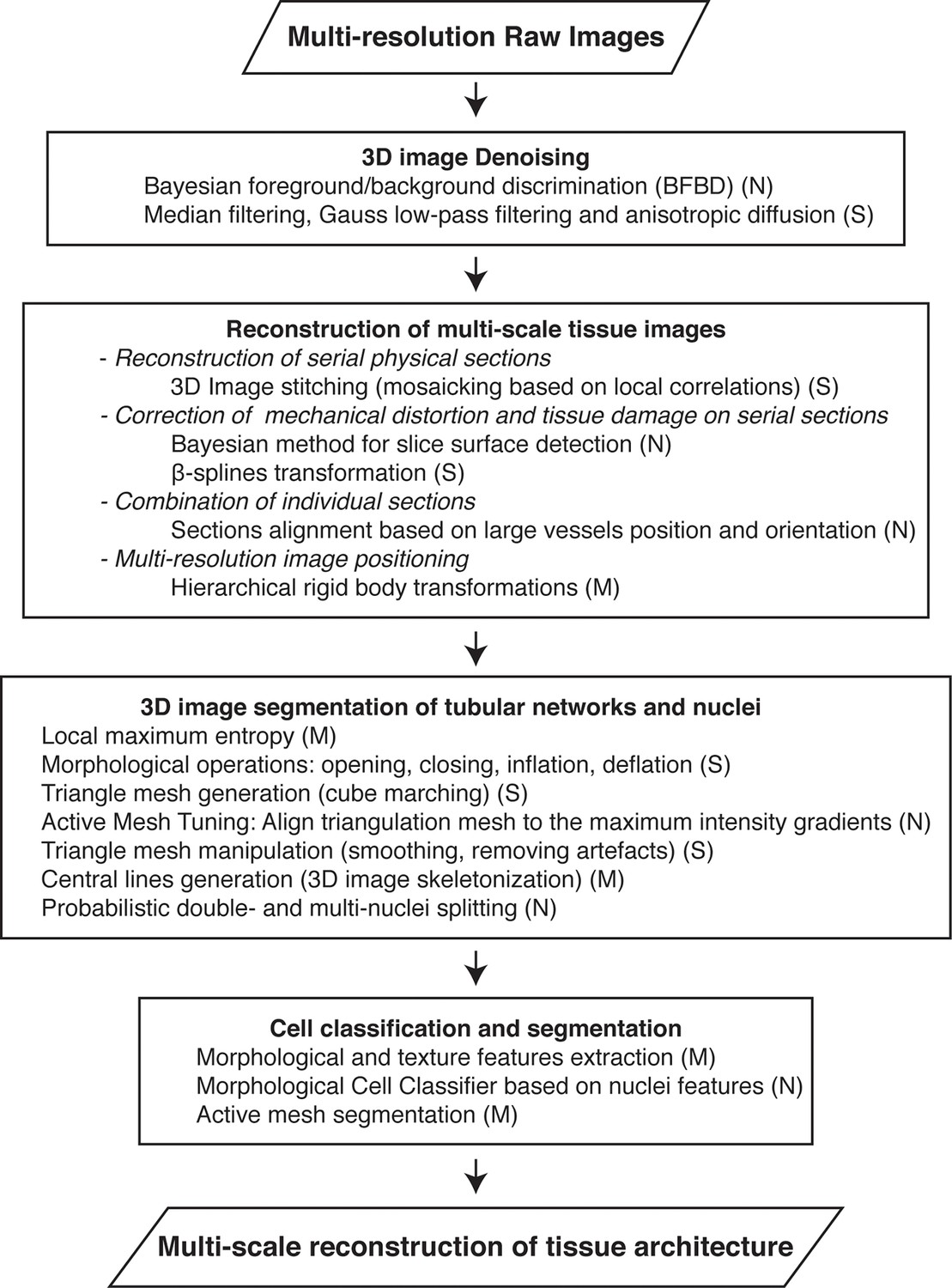
Workflow for the multi-scale reconstruction of tissue architecture from multi-resolution confocal microscopy images.
The necessary methods for each step (implemented in our software) are listed. They include newly developed ones (N) as well as standard image analysis algorithms (S) and modified versions of them (M).
Figure 1—figure supplement 2
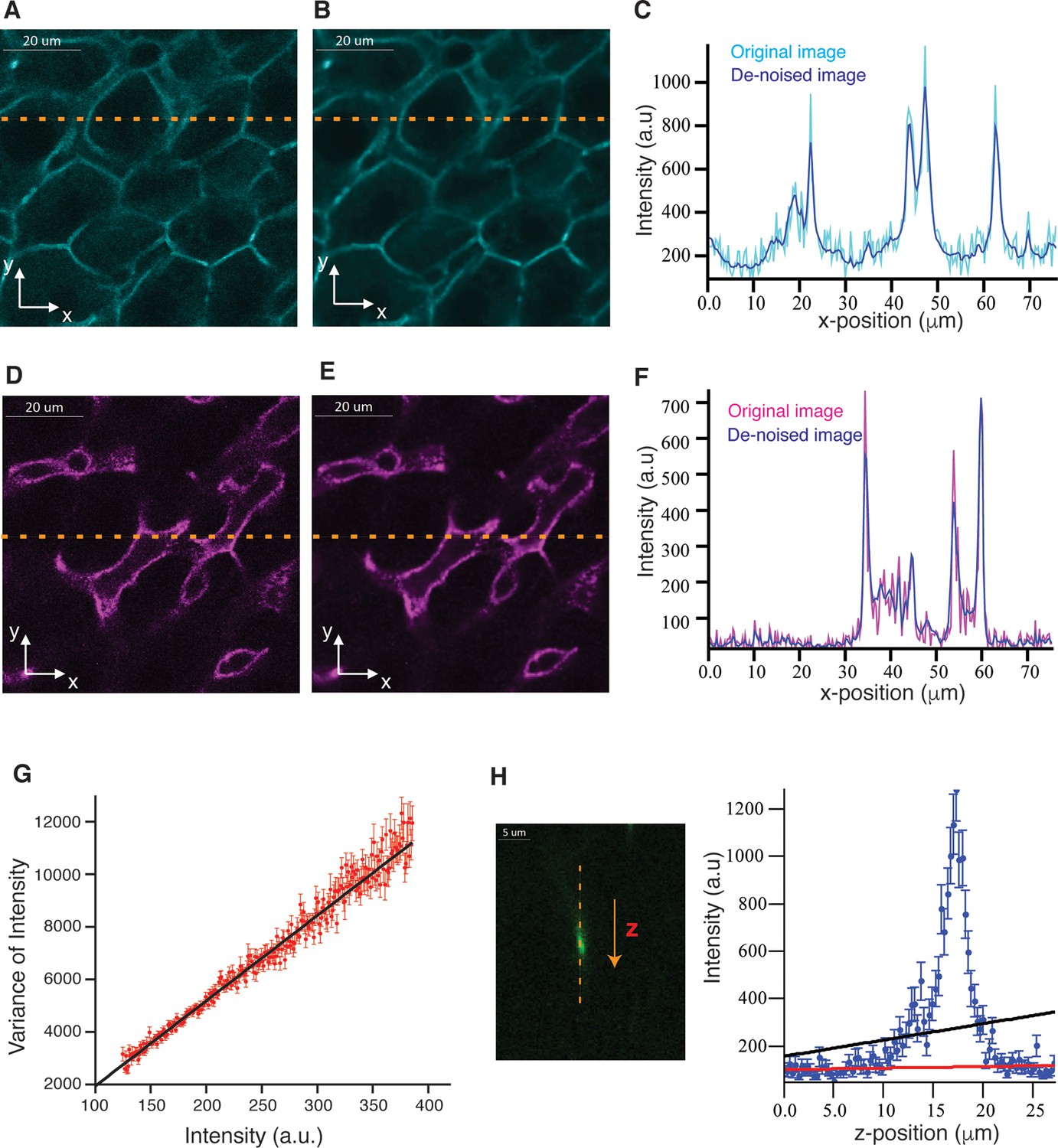
Probabilistic image de-noising algorithm for 3D images.
Single 2D plane of a high-resolution image stained with phalloidin for actin (cell borders) and Flk1 for sinusoids (A, D) before and (B, E) after applying our probabilistic image de-noising algorithm. The outlier-tolerant estimation of the background was done using a 10-pixel window. (C, F) Phalloidin/Flk1 intensity values of pixels along the horizontal yellow line for both, the original and the de-noised images. Our probabilistic image de-noising algorithm efficiently reduces the noise while preserving the edges present in the image even in the presence of high diffusive background. (G) Mean variance for each intensity level (I). The experimental data are represented by the red dots, the error bar represents SEM and the theoretical curve (straight line) is represented by the solid black line. (H) Prediction of the background intensity using linear fitting by least-squares method (solid black line) and the outlier-tolerant algorithm (solid red line) for a set of sequential intensities in z-direction (blue dots). The dots represent the intensity values of the voxels along the vertical yellow line at the original image on the left [stained with CD13 for bile canalicular (BC) network].
Figure 1—figure supplement 3
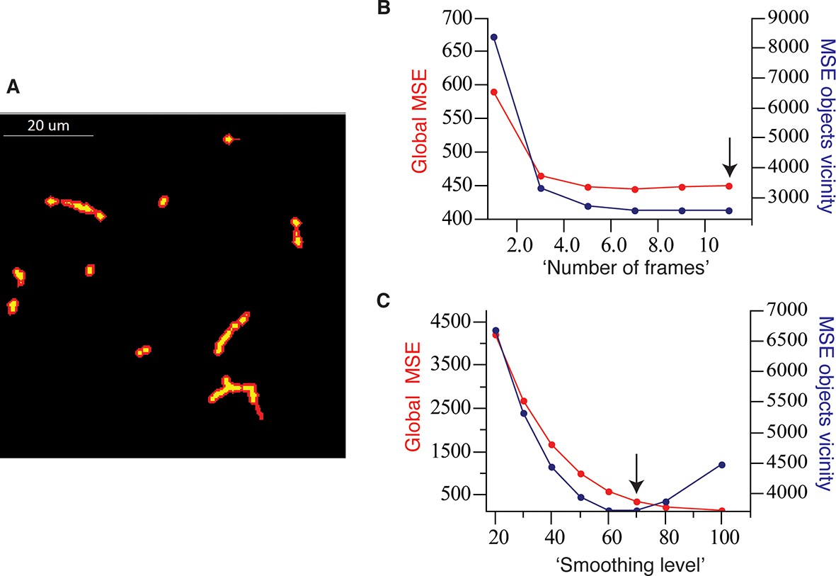
Optimal parameter selection.
(A) The mask defining the objects vicinity in the case of bile canalicular (BC) network (yellow) is shown in red and was created by applying an inflation of two voxels (~0.5 µm) to the original objects. (B) Selection of the best parameters for the ‘pure denoise’ method. We used as fixed parameter the number of cycles (10, the maximum possible). ‘Number of frames’ = 11 (the maximum available in the plug-in) shows the best results, i.e., minimum global mean square error (MSE) as well as MSE in the vicinity of the objects. (C) Selection of the best parameters for the ‘edge preserving de-noising and smoothing’ method. We used as fixed parameter the number of cycles (100). ‘Smoothing level’ = 70 corresponds the point before the MSE in the vicinity of the objects starts increasing while the global MSE remains low.
Figure 1—figure supplement 4
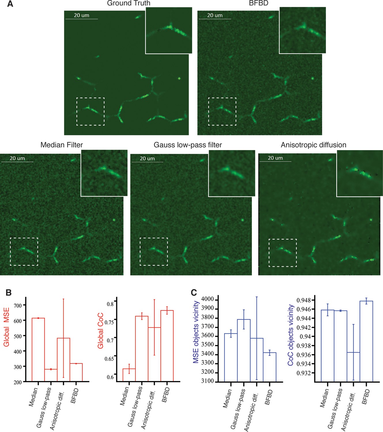
Comparison of our 3D image de-noising algorithm (BFBD) with standard methods in the field.
Panel (A) shows single 2D plane projections of an artificial high-resolution image of bile canalicular (BC) network (2:1 signal-to-noise ratio) before adding Poisson noise (ground truth) and the result of the application of our de-noising algorithm (BFBD) as well as a median filter, a Gauss low-pass filter and an anisotropic diffusion. (B) The resulting images were analysed in terms of the global mean square error (MSE) and coefficient of correlation (CoC). (C) The same metrics were evaluated only on the vicinity of the BC. Our method shows considerably better noise reduction (low global MSE and high global CoC) than the other methods, except the Gauss low-pass filter. However, the Gauss low-pass filter shows a high MSE and low CoC in the vicinity of the objects (in comparison with our method), suggesting a blurring of the object edges. The bars show the average values over three samples and the error bars correspond to standard deviations. A median filter (smooth window 3 ×3 ×3 voxels), a Gauss low-pass filter (s = 1 voxels) and an anisotropic diffusion (), where D = 0.05, α = 2, number iterations= 100, were applied.
Figure 1—figure supplement 5
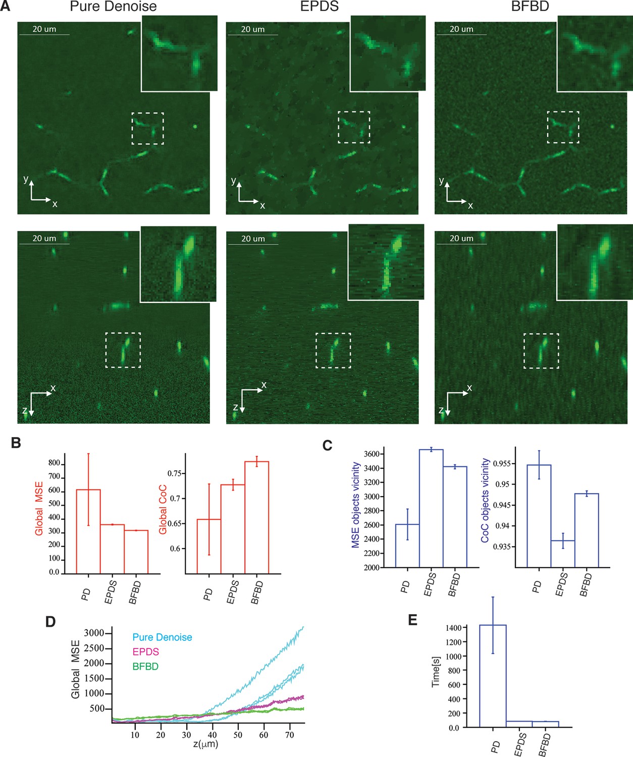
Comparison of our 3D image de-noising algorithm (BFBD) with ‘pure denoise’ (PD) (Luisier et al., 2010) and ‘edge preserving de-noising and smoothing’ (EPDS) (Beck and Teboulle, 2009).
Panel (A) shows single 2D plane projections of an artificial image of bile canalicular (BC) network (2:1 signal-to-noise ratio) after applying our de-noising algorithm as well as PD and EPDS. (B) The resulting images were analysed in terms of the global mean square error (MSE) and coefficient of correlation (CoC). (C) The same metrics evaluated only on the vicinity of the BC. Our method shows a better reduction of the noise (low global MSE and high global CoC) than the other methods. Additionally, it shows a relatively low MSE and high CoC in the vicinity of the objects. Panel (D) shows that global MSE increases with the depth of the sample for PD and EPDS, whereas it is more stable in our method. In the graph, each curve represents one independent sample. (E) Execution time of the algorithms in an Intel(R) Xeon(R) CPU E5-2620 @ 2.00 GHz. EPDS and BFBD are ~ 20 times faster than PD. The bars show the average values over three samples and the error bars correspond to standard deviations. PD and FPDS were performed using the optimal parameters shown in Figure 1—figure supplement 3. For the BFBD, we use a window of five pixels and a threshold = 1.25.
Figure 2 with 2 supplements
Reconstruction of a multi-scale lobule image.
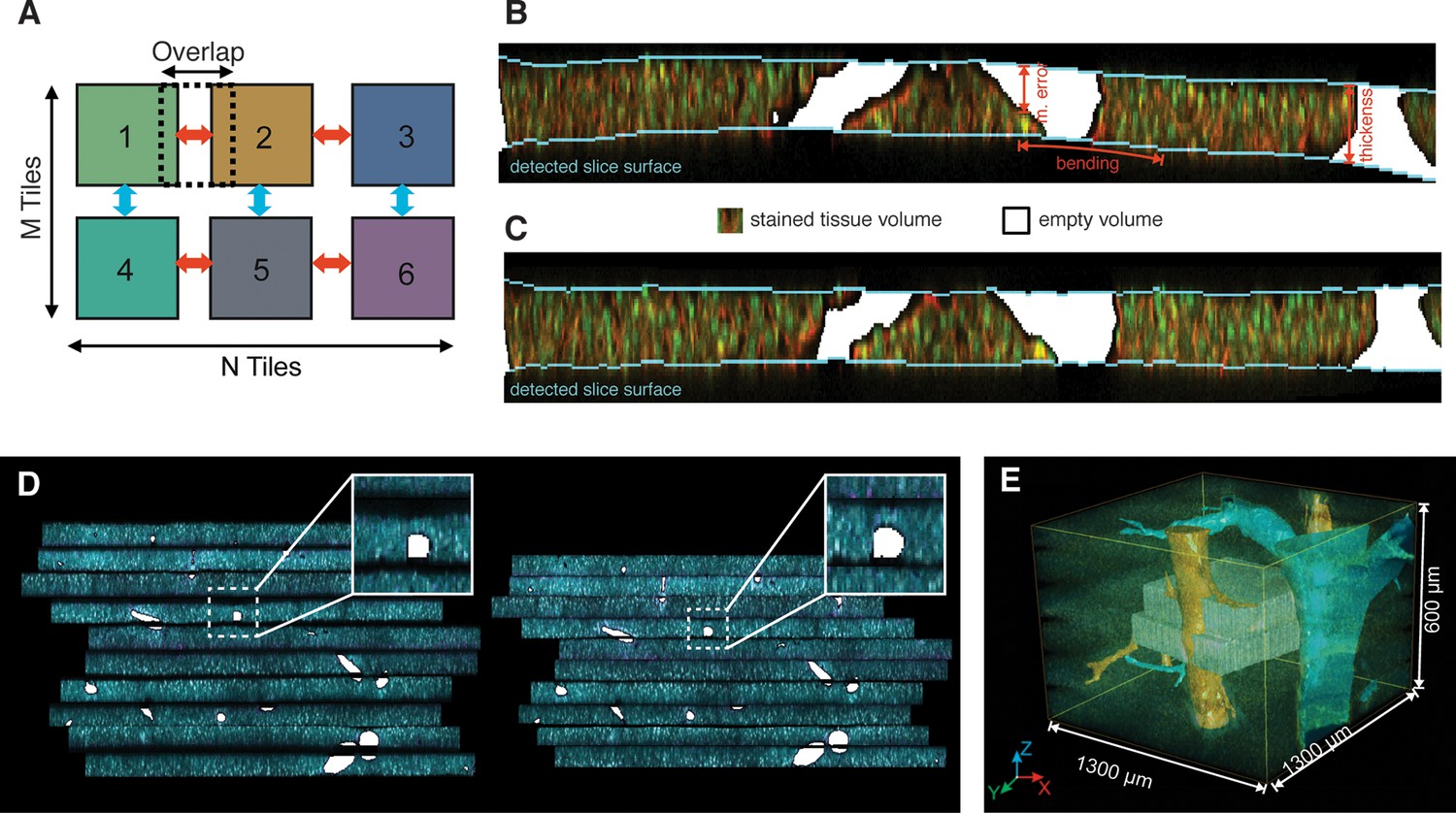
(A) Schematic representing a single serial section obtained from a grid of M × N partially overlapping 3D images (tiles). The cross-correlation between two neighbouring tiles in the grid provides a local metric, which describes the value of their relative shifts. The reconstruction of each section was performed by maximizing the sum correlations of each tile to all adjacent tiles (see ‘Methods’ for details). (B, C) Correction of tissue deformations (introduced during the sample preparation process) using a surface detection algorithm and β-spline transformation. (B) Output of the surface detection algorithm. The proposed Bayesian approach uses prior information about expected bending of the section, its thickness and measurement error (see ‘Methods’ for details) to determine the volume of the image belonging to the tissue and to the out-of-field region. (C) The tissue section after correcting its bending by using quadratic β-splines. (D) Tissue section before (left) and after (right) the correction of the mechanical distortions and the tissue damage. (E) Full lobule-level reconstruction established by the alignment of six low-resolution sections (1 μm × 1 μm × 1 μm per voxel) and the interpolation of blood vessels. Two high-resolution images (0.3 μm × 0.3 μm × 0.3 μm per voxel) were registered in the low-resolution reconstruction and are shown in grey (see Video 1).
Figure 2—figure supplement 1
Reconstruction of multi-scale tissue images.
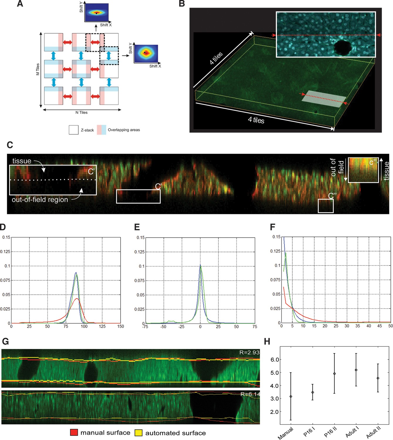
Tissue section reconstruction: (A) Schematic representation of an M × N grid of partially overlapping 3D images. The regions in light blue and light red represent the overlapping areas between neighbouring images. The colour-coded maps show the cross-correlation matrixes between neighbouring images. (B) Reconstructed tissue section from 4×4 a grid of low-resolution images. The pattern of DAPI staining (nuclei) at the intersection of two neighbouring images is shown. Correction mechanical distortion and tissue damage on serial sections: (C) x–z section of the image of a tissue section showing the main obstacles for the tissue surface detection: unstained volume of blood vessels (C') and blurring (C''). Probabilities (D) , (E) and (F) calculated from the maximum entropy segmentation (red), model equations (blue) and manual solution (green). All distributions in the figure were averaged over all tissue sections in the benchmark. (G) Comparison of manual and automated surfaces calculated for two tissue sections from P16 (upper) and adult (lower) mice datasets. (H) Accuracy of surface detection. Plot presenting the mean absolute deviation calculated between manually and automatically detected surfaces for 33 different tissue sections in 4 data sets. Since tissue section segmentation is ambiguous, the control experiment was conducted by segmenting the same tissue sections manually three times.
Figure 2—figure supplement 2
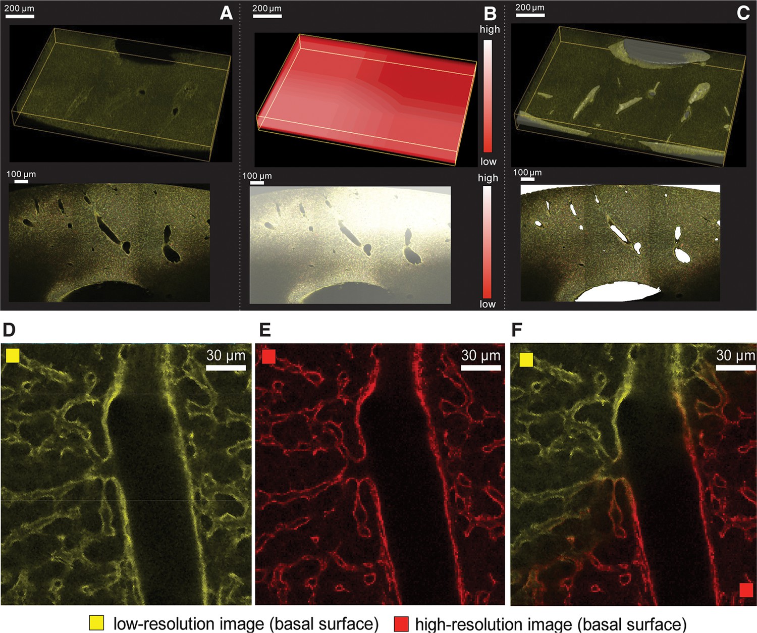
Reconstruction of multi-scale tissue images.
Tissue-level network segmentation: (A) Reconstructed image of a tissue section. Large vessels appear as empty space in the image. (B) Spatial distribution of the local maximum entropy threshold value. (C) Segmentation of large vessel in a single tissue section. Registration of high-resolution images into low-resolution ones: Representative region of a 2D plane of (D) a low-resolution (yellow) and (E) a high-resolution (red) image stained with Flk1 for sinusoids. (F) Superimposed images after the registration.
Figure 3 with 7 supplements
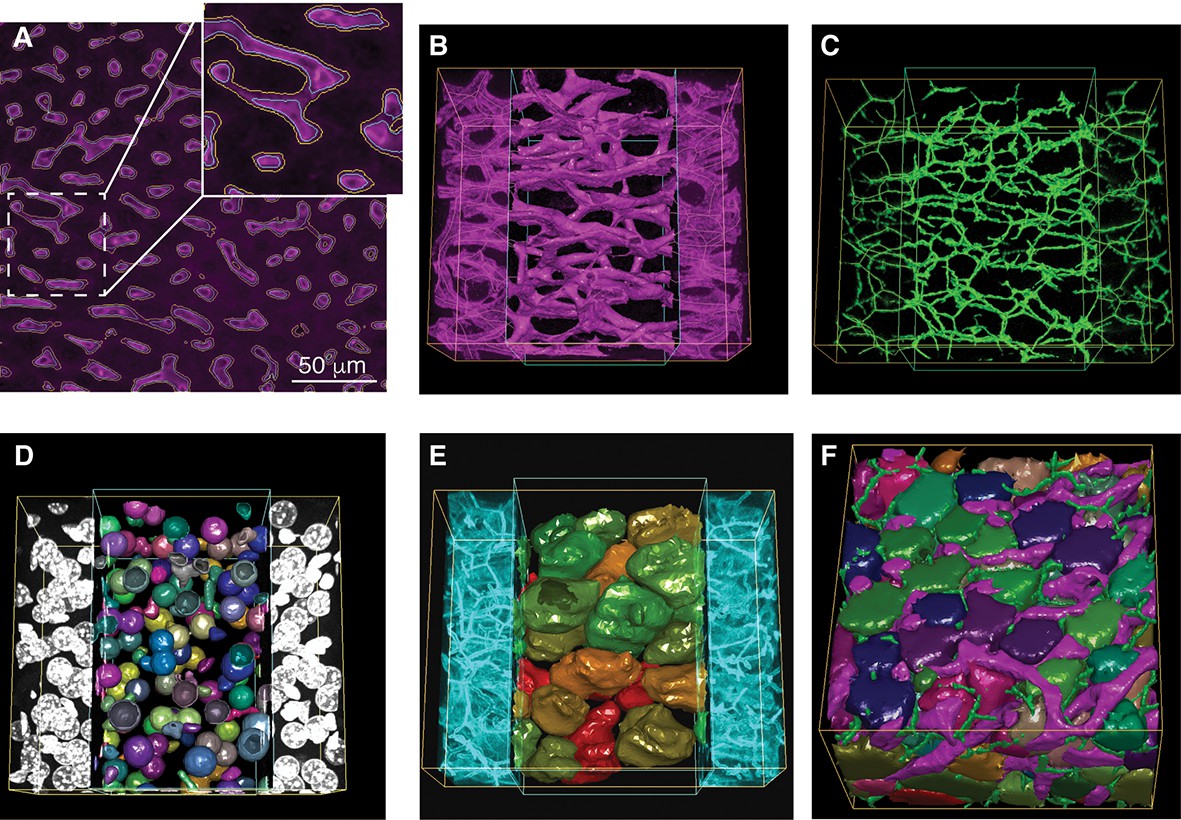
Reconstruction of tubular structures, nuclei and cells.
(A) A single 2D image section is shown with the contours of the sinusoidal network reconstruction overlaid on the de-noised image. The contours of the initial mesh are drawn in yellow, and the ones of the tuned mesh are drawn in cyan. (B–E) 3D representation of the different structures segmented in a sample of liver tissue: sinusoids (B), BC (C), nuclei (D) and cells (E). All the reconstructed structures are shown together in (F). The reconstructed triangle meshes are drawn inside the inner box and the raw images are outside. In the case of tubular networks (i.e. sinusoids and BC), the central lines of the structures are shown together with the raw images.
Figure 3—figure supplement 1
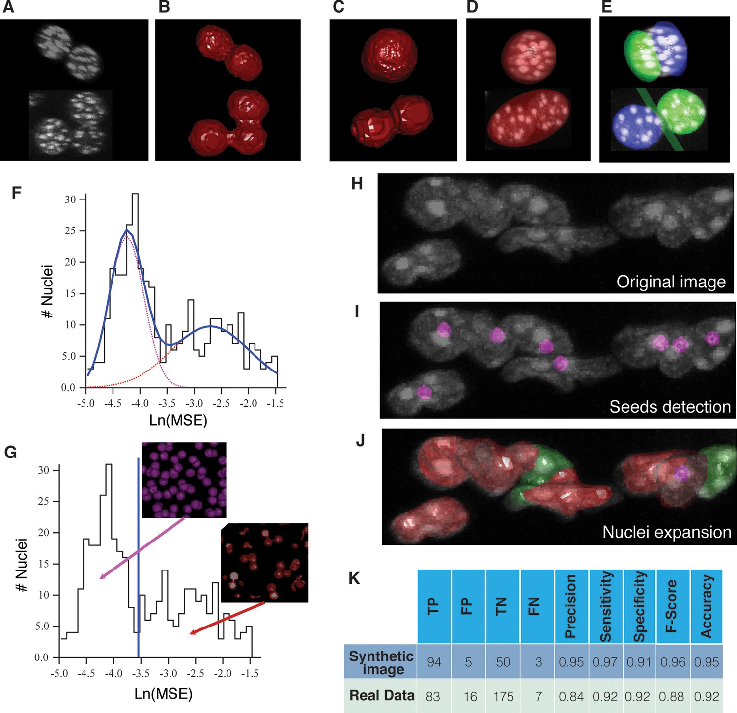
Nuclei splitting.
(A) 3D visualization of a confocal image of closely packed nuclei (DAPI). (B) Objects resulting from the initial segmentation and reconstruction: triangle meshes of the artificially merged structures. The approximation of different structures (C) by (D) one or (E) two overlapping ellipsoids is shown. Prediction of multi-nuclear structures: (F) distribution of the In(MSE) values obtained from the nuclei approximation by one and double ellipsoids. The distribution was fitted by a sum of two Gaussian distributions. The fitting curve is shown in blue (solid line) and the components in magenta and red (dash lines). (G) Calculated threshold that discriminates between bi/mono-nuclear and multi-nuclear structures. The graphs were obtained from the analysis of a sample of liver tissue, which covers the entire central vein (CV)-portal vein (PV) axis. Multi-nuclei splitting: (H) original confocal image where the nuclei seeds were detected (I) and expanded to the real nuclei shape (J). (K) The performance of the splitting algorithm was evaluated in both synthetic and real 3D images. The synthetic image consisted of 150 nuclei, which included single nuclei, double- and triple-nucleated structures. The individual nuclei had a radius between 5 and 7 µm. The multi-nucleated structures were generated with different degrees of overlap. A global background of 10% of the intensity of the nuclei was added to the whole image, then it was blurred using a Gaussian filter and finally salt and paper noise was added. The real image corresponds to an adult mouse tissue sample of 2.3 ×10⁻³ mm3 volume. The initial segmentation yielded 281 structures, which were analysed (the nuclei touching the borders of the sample were excluded from the analysis). The performance was evaluated in terms of true positive (TP), false positive (FP), true negative (TN) and false negative (FN) values. TP = correctly split, FP = over-splitting, TN = correctly not split, FN = under-splitting. Precision (PR) = TP/(TP FP), sensitivity (SN) = TP/(TP FN), specificity (SP) = TN/ (TN FP), F-score = 2 × (PR × SN)/(PR SN) and accuracy (AC) = (TP TN)/(TP TN FP FN).
Figure 3—figure supplement 2
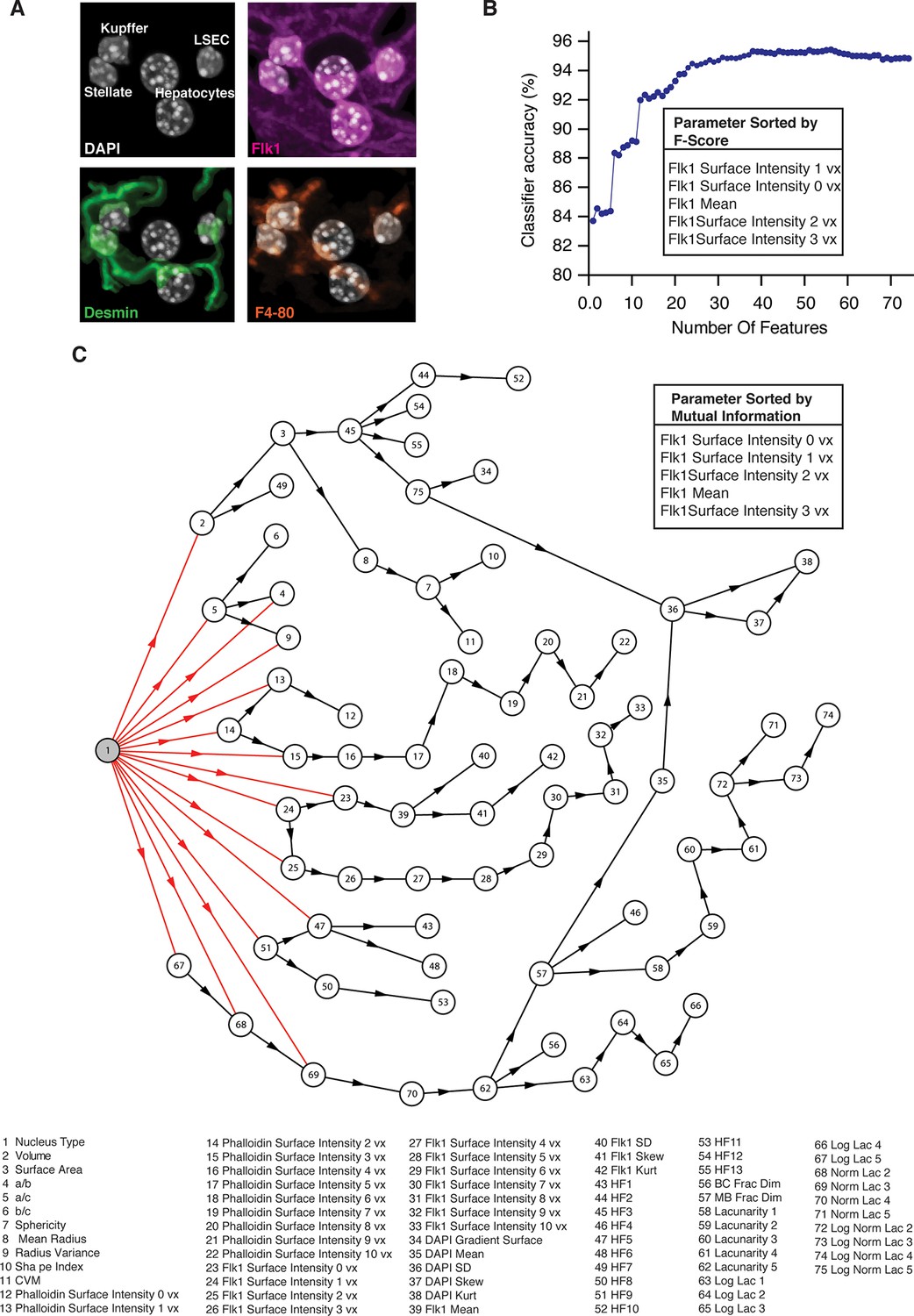
Cell classification.
(A) Example of an image used to generate the training set for the classifier. The different types of nuclei forming in liver tissue where manually classified using the specific markers, that is, Flk1 (magenta) for sinusoidal endothelial cells (SECs), the macrophage antibody F/4/80 (yellow) for Kupffer cells and the intermediate filament Desmin (green) for stellate cells. The training set was extracted from three samples covering the entire central-portal vein axis. (B) Selection of the set of parameters for the linear discriminant analysis (LDA). The 74 calculated parameters were sorted by the Fisher score and the top five ranked parameters with the largest Fisher scores are shown. The classifier accuracy in dependency of the number of parameters used for the classification is plotted. The set of parameters that yielded the highest accuracy of the classifier was chosen. (C) Features dependency obtained in the Bayesian network classifier. The Bayesian network structure learning from the experimental data revealed that 15 parameters were relevant for the nuclei classification. The five parameters with the highest mutual information to the nuclei type are shown in inset.
Figure 3—figure supplement 3
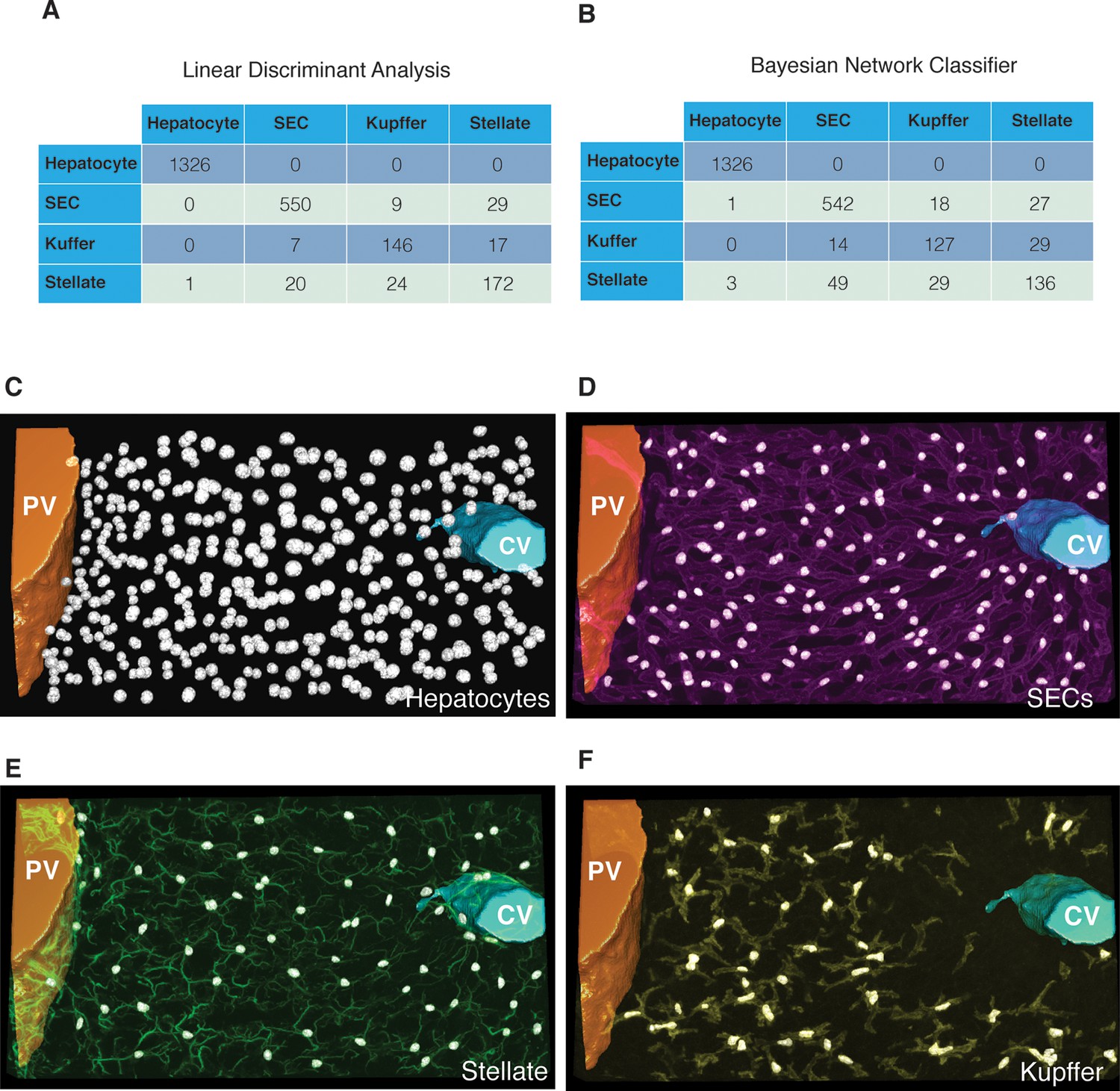
Cell classification accuracy.
Confusion matrixes obtained with the (A) linear discriminant analysis and (B) the Bayesian network classifier. The instances (e.g. nuclei) in each predicted class are represented in the columns of the matrix, while the instances in an actual class (manually identified) are represented in the rows. 3D representation of the different nuclei types identified in a representative sample of liver tissue: (C) hepatocytes, (D) sinusoidal endothelial cells (SECs), (E) stellate and (F) Kupffer cells.
Figure 3—figure supplement 4
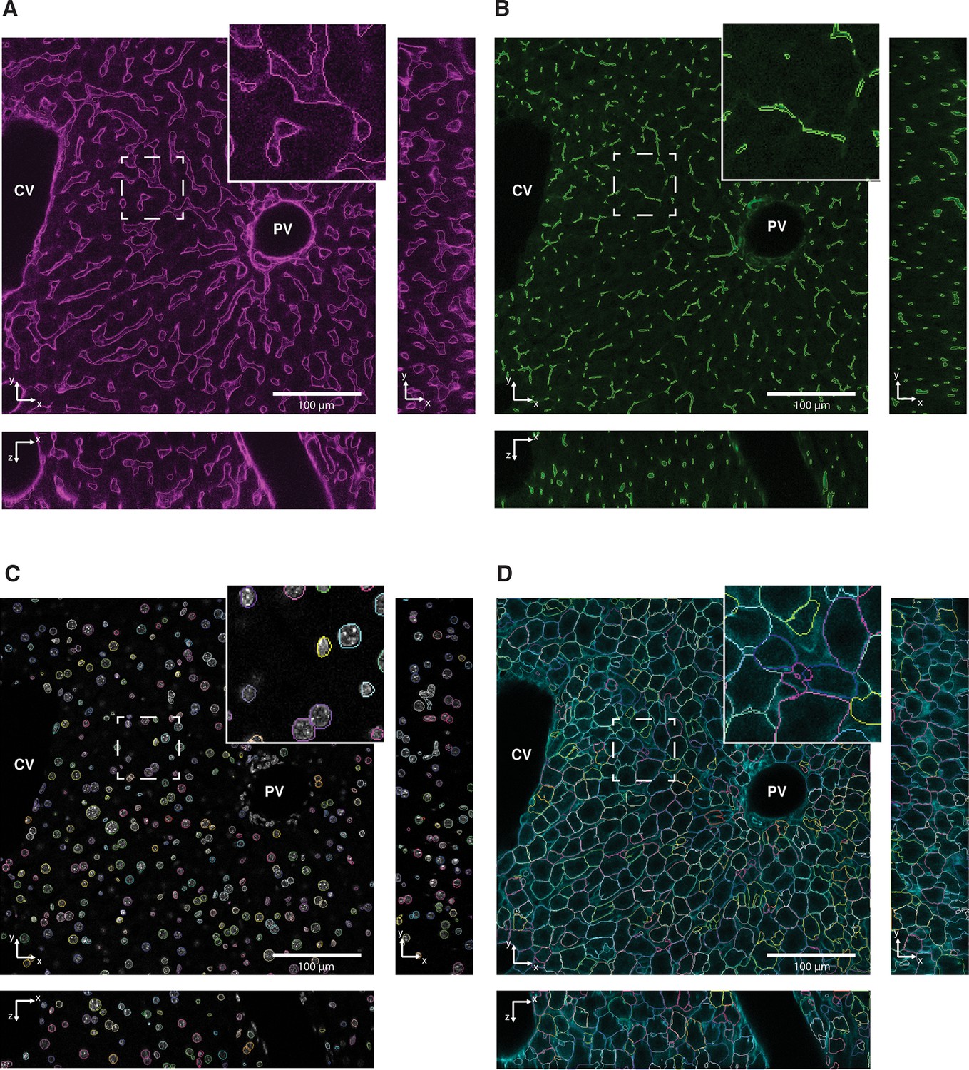
Reconstruction of tubular structures, nuclei and cells.
Single 2D image planes are shown with contours of (A) sinusoidal and (B) and bile canalicular (BC) networks, (C) nuclei and (D) cells reconstructions overlaid on raw data. Insets show zoomed areas of the image.
Figure 3—figure supplement 5
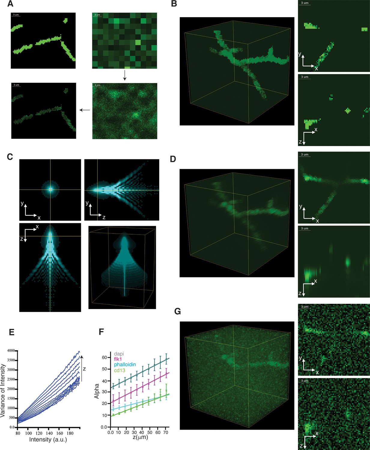
Generation of realistic 3D images of liver tissue.
(A) Generation of images with uneven staining. The image of the idealized structure (homogeneous tubes) created for the bile canalicular (BC) network is shown in the top left image. The initial coarse grained sampling (6 × 6 ×6 binning) of intensities is shown in the top-right image. The fine sampling (unbinned image) of intensities is shown in the bottom-right image and final result in the bottom-left one. (B) 3D representation and 2D projections of a model image of BC with uneven staining. (C) Characteristic point spread function (PSF) of a confocal microscope. (D) 3D representation and 2D projections of a model image of BC convolved with the PSF. (E) Mean variance of each intensity level for different depth (z-direction) levels of a confocal image. (F) Linear increase of the intensity scaling factor (alpha) with the sample depth for different channels. The error bars represent the standard deviation between three samples. (G) 3D representation and 2D projections of a final model image of BC after adding spatially variable Poisson noise.
Figure 3—figure supplement 6
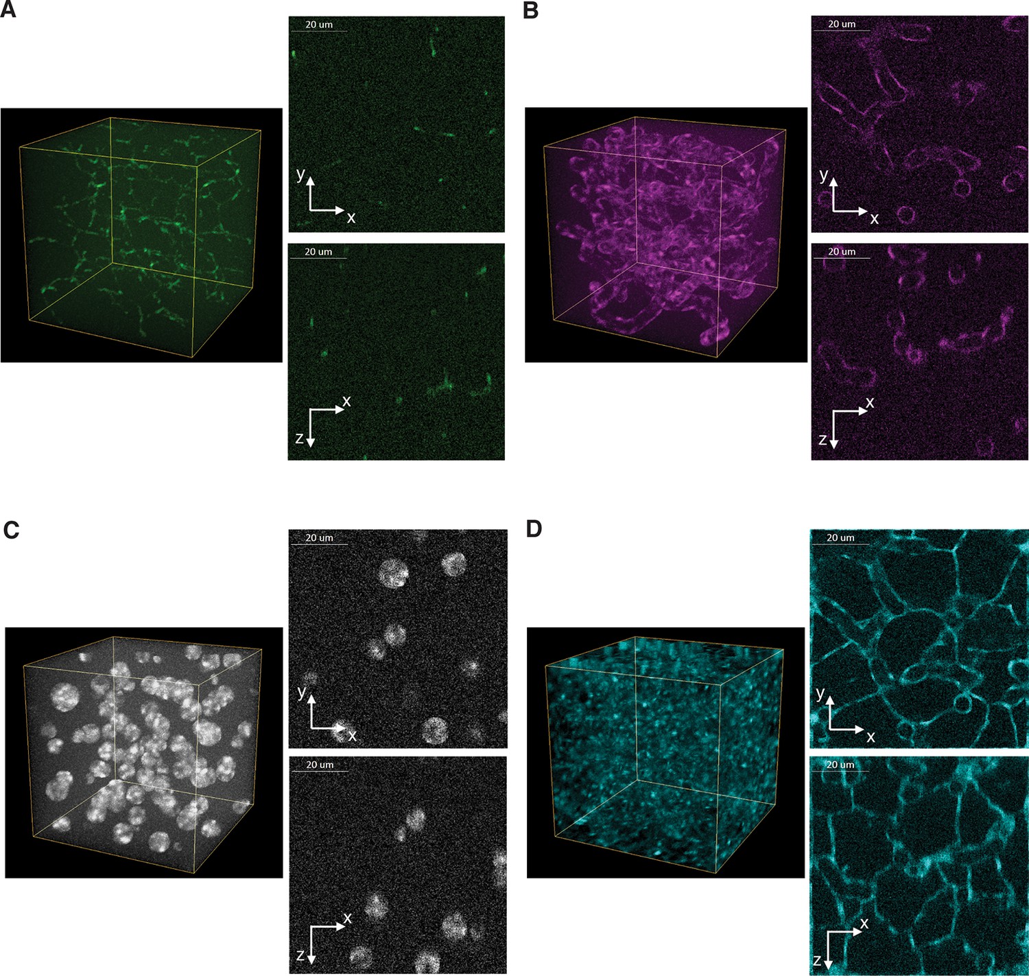
Benchmark of images to evaluate 3D reconstructions of dense tissue.
Example of a realistic 3D image of liver tissue. 3D representation and 2D projections (xy and xz) of a high-resolution image created for bile canalicular (BC) (A) and sinusoidal (B) networks as well as nuclei (C) and cell borders (D). The images size is 256 ×256 ×256 voxels with a resolution of 0.3 μm × 0.3 μm × 0.3 μm per voxel. The image shown corresponds to a 2:1 signal-to-noise ratio.
Figure 3—figure supplement 7
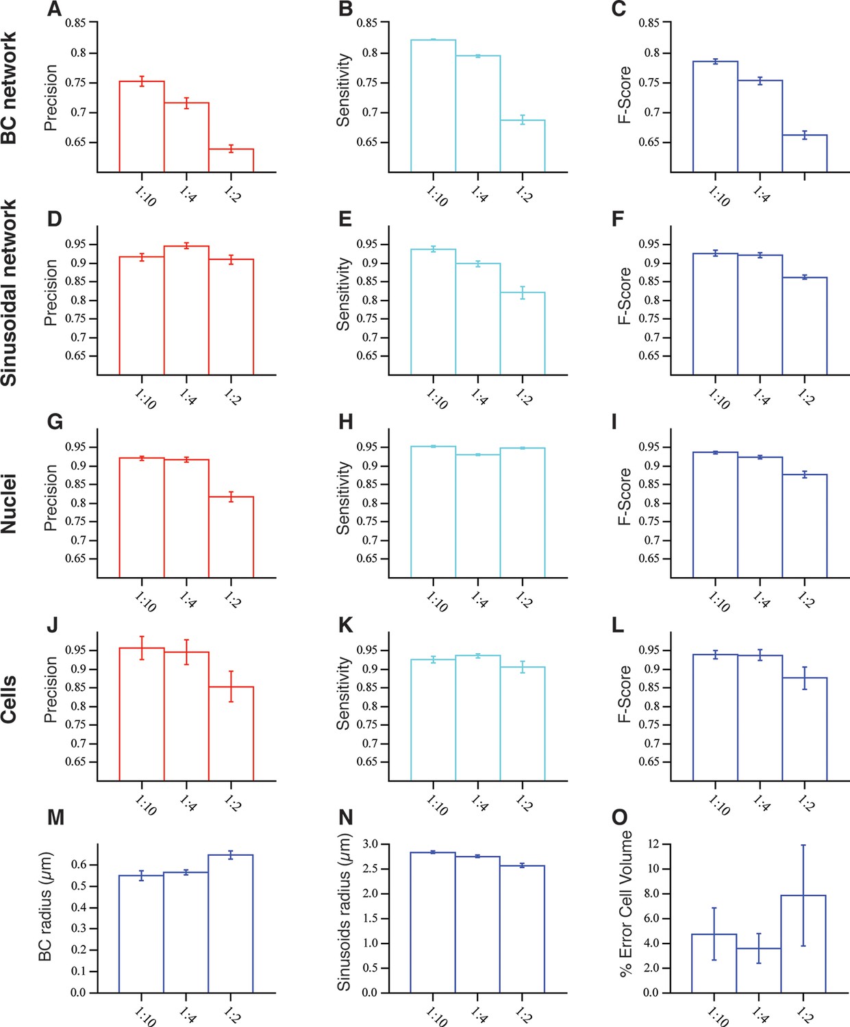
Model validation: Evaluation of the accuracy of our pipeline for the 3D reconstruction of dense tissue.
The reconstructions of the different structures forming the tissue were evaluated in terms of true positive (TP), false positive (FP), true negative (TN) and false negative (FN) values extracted from the comparison of the reconstructed image and the ground truth (image without distortions). The precision (PR) and sensitivity (SN) are defined as TP/ (TP FP) and TP/ (TP FN), respectively. F-score is given 2 × (PR × SN)/ (PR SN). The tests were performed in three sets of images (three images per set) with different signal-to-noise ratio (10:1, 4:1, 2:1). (A–C) and (D–F) The results for the bile canalicular (BC) and sinusoidal networks, respectively. (G–I) and (J–L) The ones for nuclei and cells, respectively. Whereas in the case of BC, sinusoids and nuclei, the error bar corresponds to standard deviations of the values between three images, for the cells the error bar corresponds to the standard deviation of the values over all the cells in the samples (32 cells). Only the cells that were not in contact with the boundary of the image were analysed. (M–N) The mean values for the radius of BC and sinusoidal networks. (O) The mean error in the estimation of the cell volume. The error was calculated as , where Vs and Vgt are the volumes of the reconstructed and ground truth cells, respectively.
Figure 4 with 2 supplements
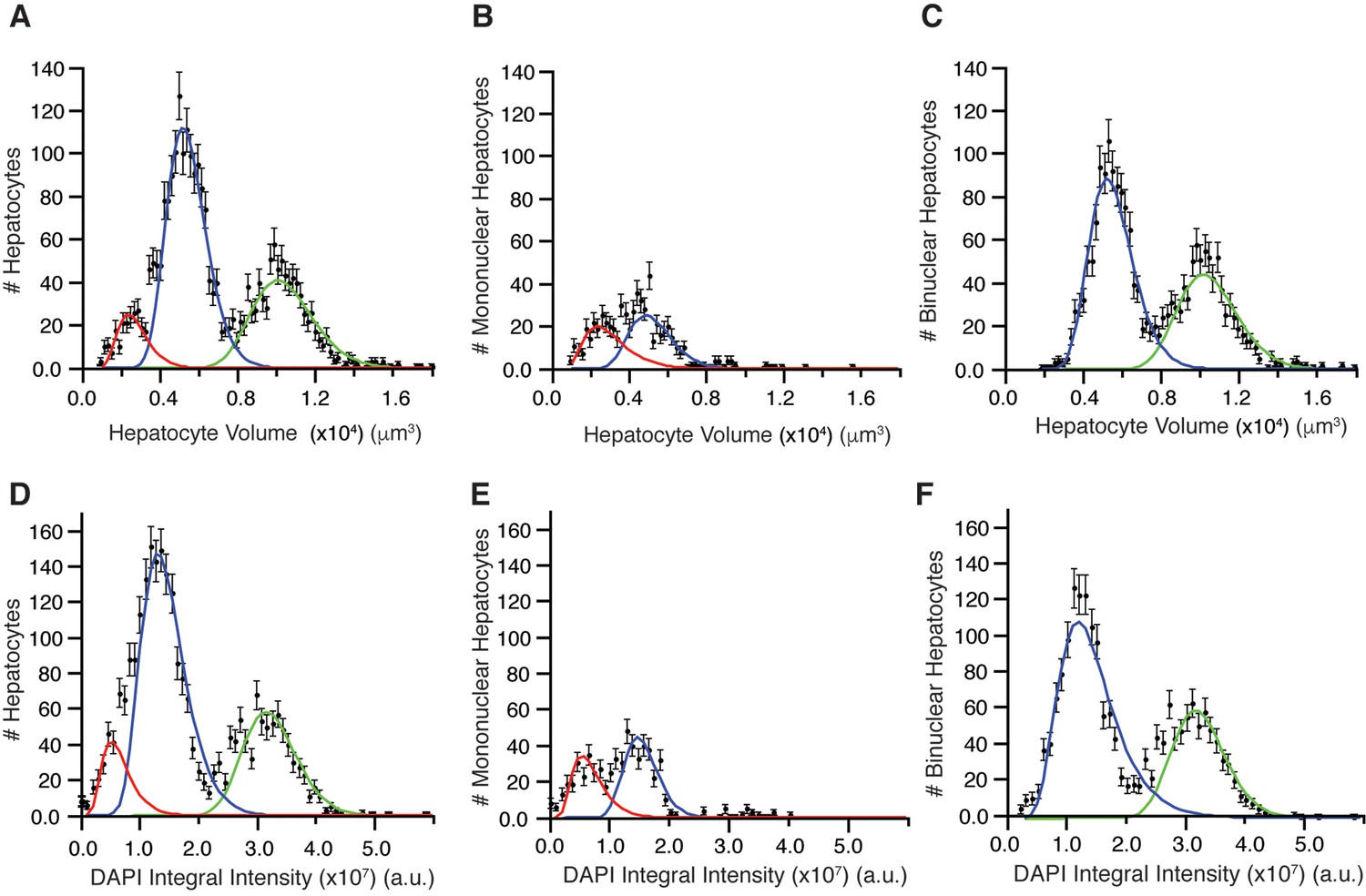
Distribution of hepatocyte volumes and DAPI integral intensity per cell for all hepatocytes (A, B) and separated by number of nuclei (B, C and E, F).
Whereas experimental data are shown by dots, the log-normal components fitted to data are shown by solid lines. (A) Cell volume distribution of all hepatocytes. (B, C) Cell volume distribution obtained for mono and bi-nucleated hepatocytes, respectively. (D) Distribution of DAPI integral intensity (proportional to the content of DNA) of all hepatocytes. (E, F) Distributions of DAPI integral intensity obtained for mono and bi-nucleated hepatocytes, respectively. The analysis was performed on 2559 hepatocytes (excluding boundary cells) from three adult mice.
Figure 4—figure supplement 1
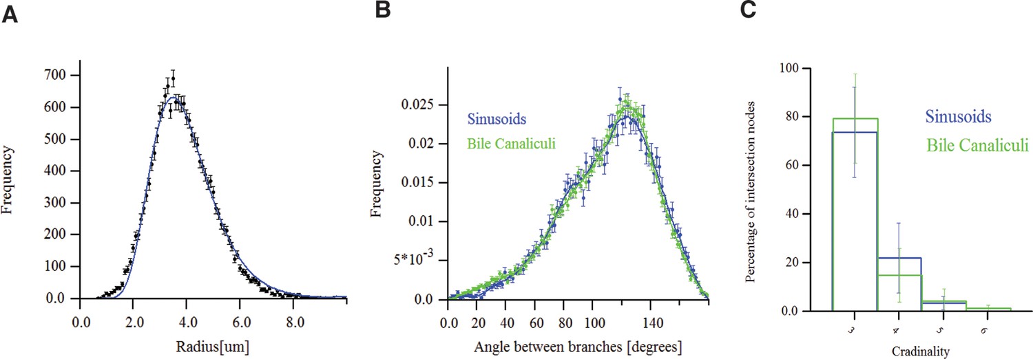
Morphometric features of the sinusoidal and bile canalicular (BC) networks.
(A) Radius distribution of the sinusoidal capillary network. (B) Distributions of the angles between branches of BC and sinusoidal networks. (C) Cardinality of branching nodes of BC and sinusoidal networks. The data shown here correspond to a representative sample of adult mouse liver.
Figure 4—figure supplement 2
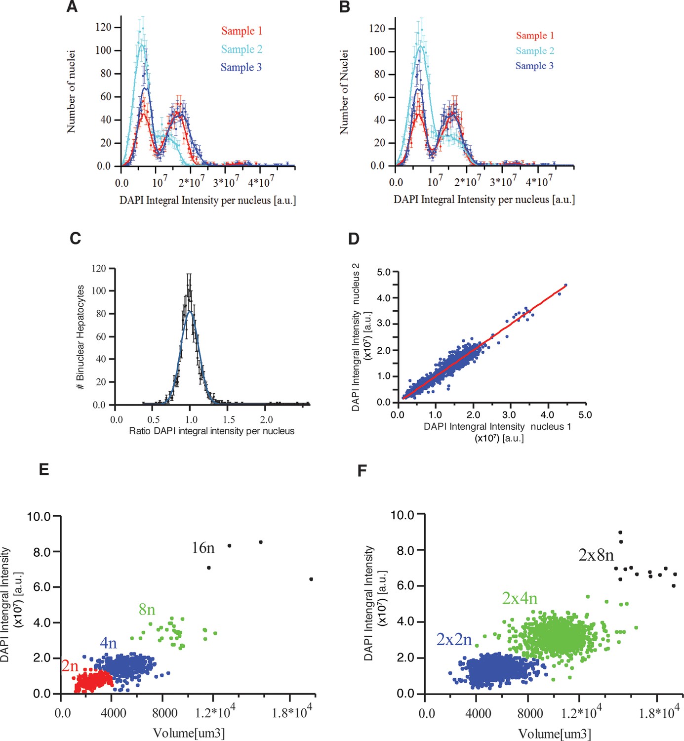
(A, B) DAPI integral intensity normalization.
Distribution of DAPI integral intensity per nucleus calculated for each sample (A) before and (B) after normalization. We found scaling (stretching) factors 1.19 and 0.93 for the second and third samples, respectively. (C, D) DNA content in bi-nuclear hepatocytes. DAPI integral intensity per nucleus was calculated for each nucleus of the cells. (C) The distribution of the ratio between DAPI integral intensity of the two nuclei in each cell. It follows a normal distribution with mean value 1.0 ± 0.21 (mean ± SD). (D) The dependency between DAPI integral intensity of the two nuclei in bi-nuclear cells. They show a linear dependency (R2 = 0.945433) with a slope of 0.995, showing that both nuclei have the same DNA content in bi-nuclear hepatocytes. (E, F) Scatter plot of the volume versus DAPI integral intensity of (E) mono-nuclear and (F) bi-nuclear hepatocytes. The results of the hierarchical clustering of (E) mono-nuclear and (F) bi-nuclear hepatocytes are shown. Four (2n, 4n, 8n, 16n) and three (2×2n, 2×4n, 2×8n) populations were found for mono-nuclear and bi-nuclear hepatocytes, respectively. The classification was performed using volume and DAPI integral intensity per cell. We used an agglomerative hierarchical cluster algorithm and tested several distances for the dissimilarity calculation and different methods for the clustering. We found that the standardized Euclidean distance with the Ward method yielded the best results.
Figure 5
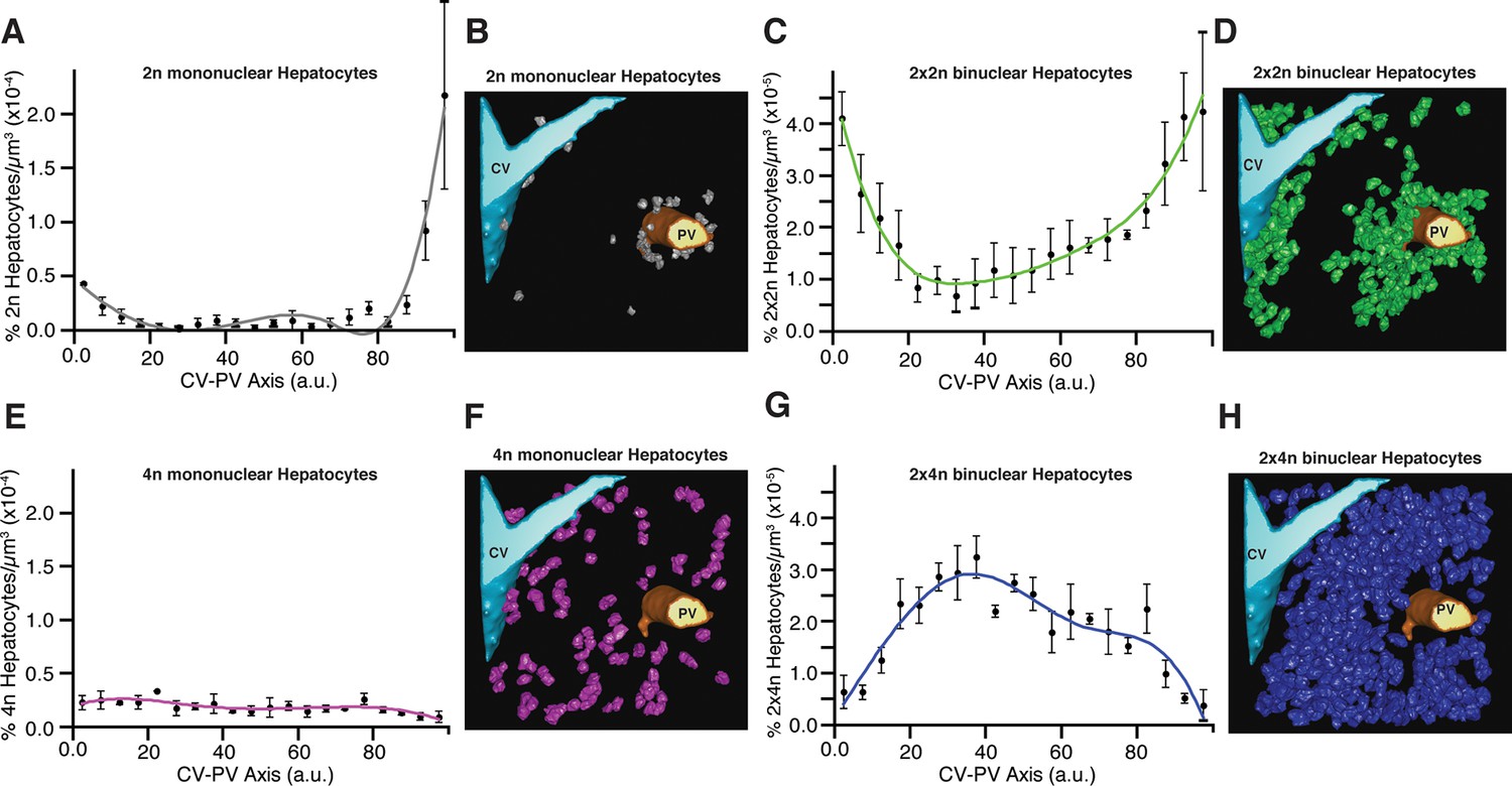
Relative density of different sub-populations of hepatocytes as function of central vein (CV)-portal vein (PV) axis coordinate.
(A, C, E, G) Relative density of 2n mono-nucleated, 2x×2n bi-nucleated, 4n mono-nucleated, 2x×4n bi-nucleated hepatocytes, respectively. (B, D, F, H) 3D visualization of the corresponding sub-populations of hepatocytes. The analysis was performed on 2559 hepatocytes (excluding boundary cells) from three adult mice. The CV-PV axis is determined by the coordinate χ, which describes the position of a point relative to the closest CV and PV. , where dcv and dpv are the distances to the closest CV and PV respectively, and D is the CV-PV distance. χ takes values between 0 and 100, where 0 and 100 represents a localization at the CV and PV surfaces, respectively.
Figure 6 with 2 supplements
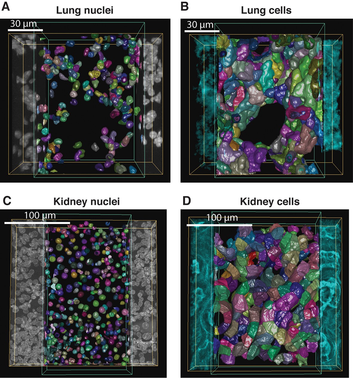
Reconstruction of geometrical models of lung and kidney tissues.
3D representation of the different structures segmented in each tissue: (A, C) nuclei and (B, D) cells in the lung and kidney tissues, respectively. The triangle meshes are drawn inside the inner box and the raw images outside.
Figure 6—figure supplement 1
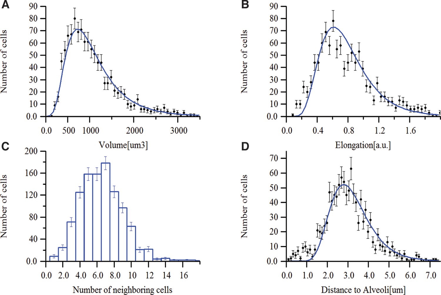
Morphometric features of lung tissue.
Distributions of (A) volume, (B) elongation and (C) number of neighbouring cells for the lung cells. (D) Distribution of the cell position (centre of the cell) relative to the closest alveoli.
Figure 6—figure supplement 2
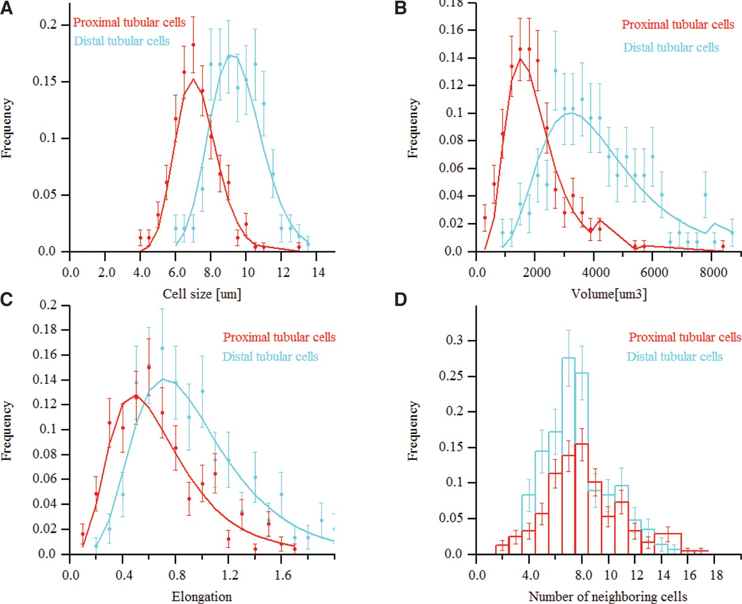
Morphometric features of kidney tissue.
(A) and (B) The size and volume distribution of the two cell types identified in the kidney tissue, proximal and distal tubular structures. It was observed that the two cell populations have different characteristic sizes, proximal cells were found to be larger than distal ones. (C) and (D) The distribution for the cells elongation and the number of neighbouring cells, respectively.
Author response image 1
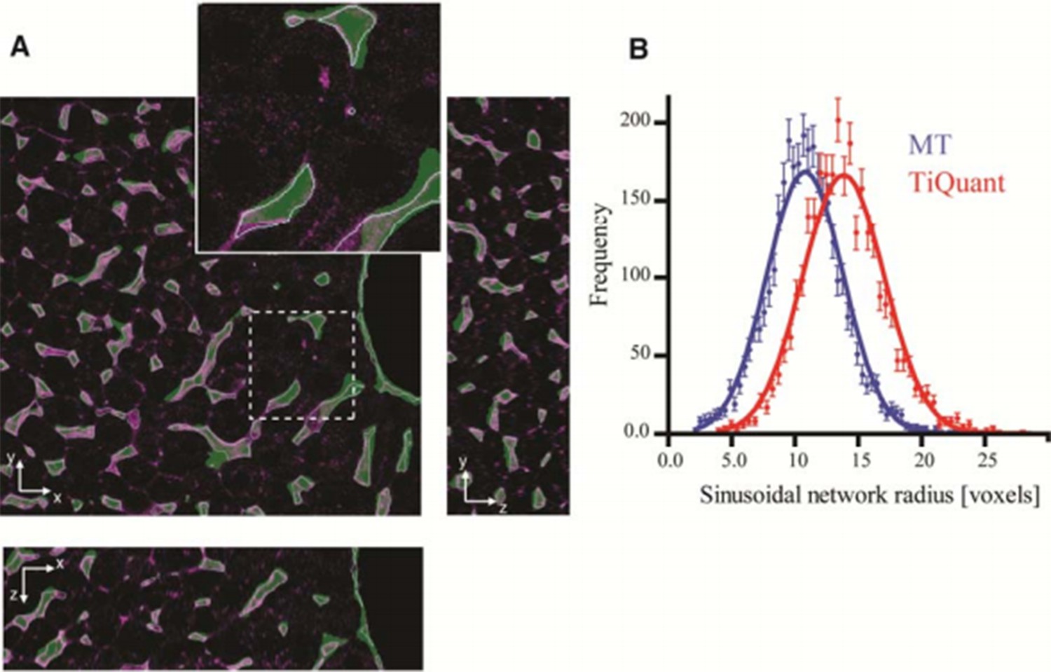
Comparison of our pipeline with TiQuant (Hammad et al., 2014, Friebel et al., 2015) applied on the reconstruction of liver tissue.
Our image analysis pipeline (MT) was applied on the dataset provided as a test for TiQuant ( http://ms.izbi.uni-leipzig.de/index.php/software). Panel (A) shows single 2D plane sections of a liver tissue image stained for sinusoids (magenta), whereas the segmentation generated by TiQuant (provided within the dataset) is shown as a partially transparent (green) image overlapping with the original one. Our reconstructions are shown as object contours (magenta lines). Panel (B) shows the radius distributions of the sinusoidal network extracted from reconstructions provided by TiQuant (red) and generated by the MT pipeline (blue). The estimated value of the radius is expressed in voxels since no information about the voxel size is provided. Each histogram was fit by a Gaussian distribution (with mean 14.08 and 11.00, for TiQuant and MT, respectively). The dots correspond to the extracted data and the solid lines to the corresponding fits. Our active mesh tuning approach yielded radius estimation for the sinusoidal network ~20% smaller than the voxel-based methods of TiQuant. These results are in line with the ones obtained from our experimental data.
Videos
Video 1
3D image visualization of a multi-resolution geometrical model of liver tissue.
A set of six low-resolution (1.0 μm × 1.0 μm × 2.0 μm per voxel) and two high-resolution tissue sections (0.3 μm × 0.3 μm × 0.3 μm per voxel) were used. Central veins are shown in light blue, portal veins in orange and high-resolution cubes in grey.
Video 2
Reconstruction of all imaged structures in a high-resolution image.
A 2x2 stitched (~ 400 μm × 400 μm × 100 μm) high-resolution image (0.3 μm × 0.3 μm × 0.3 μm per voxel) was used. First, the reconstruction of the large vessels, that is, central vein (CV) (cyan), portal vein (PV) (orange) and bile duct (green) are shown. Then, raw images and the corresponding reconstructed objects of the different structures are shown sequentially: sinusoids (magenta), BC (green), nuclei (random colours) and cells (random colours). Additionally, central lines are shown for the tubular structures. Finally, all segmented structures are shown. This video provides a complete over view of the reconstructed objects in a typical high-resolution image.
Video 3
Detailed reconstruction of all imaged structures in a high-resolution image.
In order to highlight the details of the reconstruction of small structures [e.g. nuclei, bile canalicular (BC) network, etc.], a video of a small, cropped (~125 μm × 125 μm × 75 μm) high-resolution image (3 μm × 0.3 μm × 0.3 μm per voxel) was generated. Similarly to Video 2, the raw image and the corresponding reconstructed structures of sinusoids (magenta), BC (green), nuclei (random colours) and cells (random colours) are shown sequentially.
Video 4
3D reconstruction of lung tissue.
Nuclei and cells reconstructed from a high-resolution image (∼220 μm × 220 μm × 80 μm). First, the raw images of the cell cortex (F-actin by phalloidin) and nuclei (DAPI) staining are displayed. Then, the reconstruction of the nuclei (random colours) and the cells (random colours) are shown.
Video 5
3D reconstruction of kidney tissue.
Nuclei and cells reconstructed from a high-resolution image (∼220 μm × 220 μm × 80 μm). First, the raw images of the cell cortex (F-actin by phalloidin) and nuclei (DAPI) staining are displayed. Then, the reconstruction of the nuclei (random colours) and the cells (random colours) are shown.
Tables
Table 1
List of the 74 parameters calculated for the nuclei classification.
| Parameter | F-score | Parameter | F-score |
|---|---|---|---|
| FLK1 surface intensity 1 vx | 4.802 | Mean radius | 0.920 |
| FLK1 surface intensity 0 vx | 4.737 | FLK1 KURT | 0.915 |
| FLK1 mean | 4.674 | MB Frac Dim | 0.904 |
| FLK1 surface intensity 2 vx | 4.570 | Log Lac2 | 0.885 |
| FLK1 surface intensity 3 vx | 4.100 | HF2 | 0.833 |
| Phallo surface intensity 2 vx | 3.477 | HF13 | 0.825 |
| FLK1 surface intensity 4 vx | 3.453 | HF3 | 0.817 |
| Phallo surface intensity 1 vx | 3.430 | Phallo surface intensity 9 vx | 0.787 |
| FLK1 SKEW | 3.351 | Surface area | 0.768 |
| Phallo surface intensity 3 vx | 3.253 | Log lac 3 | 0.718 |
| Phallo surface intensity 0 vx | 3.236 | Radius variance | 0.669 |
| Norm lac 3 | 2.930 | Volume | 0.668 |
| Norm lac 2 | 2.913 | BC Frac Dim | 0.649 |
| FLK1 surface intensity 5 vx | 2.857 | Log lac 4 | 0.612 |
| Norm lac 4 | 2.847 | Phallo surface intensity 10 vx | 0.554 |
| Phallo surface intensity 4 vx | 2.838 | Log lac 5 | 0.536 |
| Norm lac 5 | 2.753 | Sphericity | 0.423 |
| Phallo surface intensity 5 vx | 2.347 | HF7 | 0.408 |
| FLK1 surface intensity 6 vx | 2.310 | Shape index | 0.402 |
| HF9 | 2.141 | Lacunarity 1 | 0.381 |
| FLK1 surface intensity 7 vx | 1.893 | b/c | 0.342 |
| Phallo surface intensity 6 vx | 1.868 | Lacunarity 2 | 0.333 |
| HF5 | 1.575 | Lacunarity 3 | 0.309 |
| HF8 | 1.554 | Lacunarity 4 | 0.295 |
| FLK1 surface intensity 8 vx | 1.552 | HF4 | 0.287 |
| HF11 | 1.471 | Lacunarity 5 | 0.285 |
| Phallo surface intensity 7 vx | 1.444 | HF12 | 0.153 |
| a/c | 1.406 | DAPI Sd | 0.123 |
| Log lac 1 | 1.287 | DAPI gradient surface | 0.094 |
| FLK1 surface intensity 9 vx | 1.265 | Log norm lac 2 | 0.087 |
| HF6 | 1.158 | CVM | 0.076 |
| Phallo surface intensity 8 vx | 1.084 | Log norm lac 3 | 0.062 |
| FLK1 surface intensity 10 vx | 1.018 | Log norm lac 4 | 0.045 |
| HF1 | 0.978 | DAPI SKEW | 0.035 |
| FLK1 Sd | 0.942 | Log norm lac 5 | 0.033 |
| HF10 | 0.939 | DAPI mean | 0.029 |
| a/b | 0.937 | DAPI KURT | 0.022 |
-
Note: The parameters are sorted based on their Fisher score, which is a measure of the discriminative power of the parameter.
Table 2
Internal consistency of the sinusoidal network data.
| Sample | Vs | Ls/(mm/mm3) | rs/(mm × 103) | Vc ∼ π × rs2 × Ls | Vc/Vs |
|---|---|---|---|---|---|
| 1 | 0.16 | 2853.4 | 4.05 | 0.15 | 0.92 |
| 2 | 0.14 | 2976.4 | 3.75 | 0.13 | 0.95 |
| 3 | 0.20 | 3505.8 | 4.50 | 0.22 | 1.09 |
| Hammad et al., 2014 | 0.15 | 5400.0 | 4.80 | 0.39 | 2.55 |
-
Notes: The fraction of volume of the sinusoids (Vs), the length of the sinusoidal network per volume unit (Ls) and the average radius of the network (rs) were measured independently for each sample. A theoretical approximation of the fraction of volume of the sinusoids (Vc), considering it consists of ideal cylinders, was calculated (Vc ∼ π × rs2 × Ls). Then, the ratio between the measured and the calculated fractions of volume (Vc/Vs) was calculated. Values close to 1.0 reflect auto consistency on the data. We performed the same calculation with the data reported in Hammad et al. (2014).
Additional files
-
Supplementary file 1
3D ‘ground truth’ voxelated model of liver tissue (0.3 μm × 0.3 μm × 0.3 μm per voxel).
- https://doi.org/10.7554/eLife.11214.034
Download links
A two-part list of links to download the article, or parts of the article, in various formats.
Downloads (link to download the article as PDF)
Open citations (links to open the citations from this article in various online reference manager services)
Cite this article (links to download the citations from this article in formats compatible with various reference manager tools)
A versatile pipeline for the multi-scale digital reconstruction and quantitative analysis of 3D tissue architecture
eLife 4:e11214.
https://doi.org/10.7554/eLife.11214


