Striatal dynamics explain duration judgments
Figures
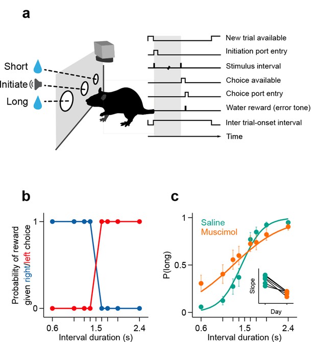
Rats judged interval durations as either long or short.
(a) Rats triggered interval stimuli (i.e. two brief auditory tones separated by a silent interval of random duration) by inserting their snout into a central port. Following interval offset, animals reported their long vs short judgment at two lateral choice ports. Correct trials yielded a water reward, while incorrect or premature responses produced a white noise sound and a time out. Top view, high-speed video was acquired throughout task performance. (b) Reward contingency. (c) Averaged psychometric curves following bilateral muscimol or saline injections in dorsal striatum (mean ± standard deviation across session means, and logistic fit; n = 3 rats, 4 sessions each). Inset: slope of psychometric curves on consecutive saline and muscimol sessions. All raw data for Figure 1 can be found in Figure 1—source data 1.
-
Figure 1—source data 1
The. txt file contains trial by trials stimulus (Interval), choice (choiceLong), animal (Name), treatment (MuscimolDose) and session (Date).
- https://doi.org/10.7554/eLife.11386.004

Histological confirmation of cannula placements.
Histology slices and schematic representation of the location of saline and muscimol injections. Coronal slices at intermediate anterior posterior (AP) positions are shown for reference at +0.84mm (left, rat Albert), +1.68 mm (center, rat Yuri) and + 0.60 mm (right, rat Zack) from Bregma. Vertical grey bars represent the location of the cannula placements. Yellow asterisks (*) show the approximate dorsal-ventral (DV) position from where the injectors extended 1.5 mm bellow the cannulae.
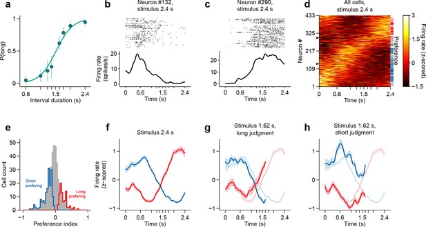
Dynamics of striatal subpopulations predict duration judgments.
(a) Psychometric function for neural recording sessions (mean ± standard deviation across sessions and logistic fit, n = 37 sessions from 3 rats). (b,c) Raster plot and peri-stimulus time histogram (PSTH) of two example cells for trials in which the longest stimulus interval (2.4 s) was presented. Time = 0 corresponds to stimulus onset. (d) Normalized PSTHs of all neurons for trials in which the longest stimulus interval was presented. Arrowheads indicate cells shown in (b,c). Blue and red ticks indicate cells with significant short and long preferences, respectively. (e) Histogram of preference indices. Blue and red outlines indicate subpopulations with significant short and long preferences, respectively. (f) Averaged, normalized PSTH of the two subpopulations outlined in (e) for trials in which the longest stimulus interval was presented (mean ± SEM). (g) Same as in (f), for trials in which a near-boundary stimulus interval (1.62 s) was judged as long. For comparison, curves shown in (f) are reproduced as a watermark. (h) same as (g) for trials in which the stimulus was judged as short. For single subjects, see Figure 2—figure supplement 2 . Behavior and neural spike count data for Figure 2 and Figure 2—figure supplements 1 and 2 can be found in Figure 2—source data 1.
-
Figure 2—source data 1
Folder with raw data for Figures 2–4.
Each file in the source data folder is named “‘<animal>_<session>"’, and contains an 8x2 cell "‘spikeCounts"’. For each of the eight stimuli and two choices, "‘spikeCounts"’ contains a matrix of spike counts with dimensions:number of neurons x number of trials x number of time steps. The stimuli (delay to the second tone in seconds) and choices are ordered as follows:STIM_SET = [0.60 1.05 1.26 1.38 1.62 1.74 1.95 2.4];CHOICES = ['incorrect' 'correct'];The spike counts are given from 500 ms prior to trial initiation up to 500 ms after the time of the second tone and were binned in 2 ms wide bins.This folder also includes underlying data for Figures 3 and 4.
- https://doi.org/10.7554/eLife.11386.007
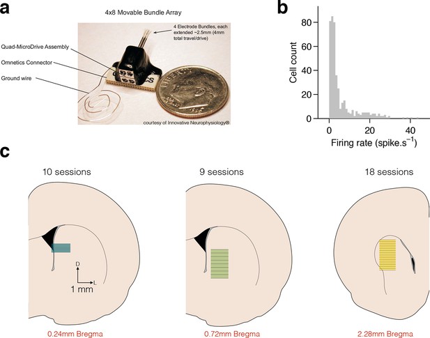
Electrophysiological recordings in dorsal striatum.
(a) Movable microwire bundle array (Innovative Neurophysiology) used for all neural recordings. (b) Histogram of firing rates for all selected cells (bin size 1 spike/s). (c) Schematic representation of the striatal recording sites. Coronal slices at intermediate AP positions are shown for reference (left to right, rats Bertrand, Edgar and Fernando). Colored rectangles show the approximate DV position of the wire bundles across recording sessions and horizontal black lines represent session by session recording sites, for 10, 9 and 18 recording sessions, respectively.
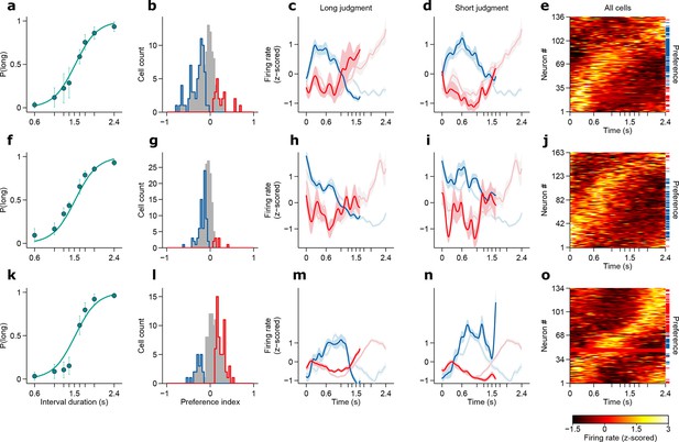
Dynamics of striatal subpopulations predict duration judgments.
(a,f,k) Psychometric functions for the recording sessions of rats Bertrand (a), Edgar (f) and Fernando (k) (mean ± standard deviation across sessions and logistic fit). (b,g,l) Histograms of preference indices for the same individual animals. Blue and red outlines indicate subpopulations with significant short and long preferences, respectively. (c,h,m) Averaged, normalized PSTHs of the two subpopulations outlined in (b,g,l) for trials in which the a near-boundary stimulus interval (1.62 s) was judged as long (mean ± SEM). (d,i,n) same as in (c,h,m) for short judgment trials. (e,j,o) Normalized PSTHs of all neurons for each animal for trials in which the longest stimulus interval was presented. Blue and red ticks indicate cells with significant short and long preferences, respectively.
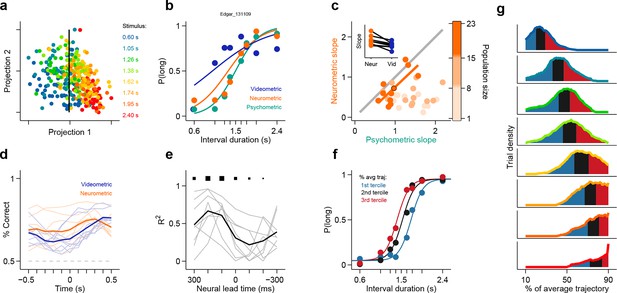
Simultaneously recorded population state at interval offset can explain behavioral performance.
(a) Low dimensional representation of population state at interval offset for one example session. Black line is the decision rule (see text). (b) Example psychometric, neurometric and videometric curves for the same session as in (a). (c) Slopes of psychometric and neurometric curves for all sessions. Color indicates terciles of population size. Highlighted data point corresponds to the session in (a-b). Inset: regression slope of neurometric and videometric curves for sessions in the upper tercile. See Figure 3—figure supplement 2 for psychometric-videometric comparison at interval offset and choice. (d) Performance of an ideal observer analysis in predicting stimulus category, applied to neural (orange) and video (blue) data obtained at different times relative to interval offset. Thin lines corresponds to individual sessions. Thick lines are averages. (e) The orange and blue curves (thin lines in panel (d)) for corresponding sessions were regressed against each other at different time shifts. The regression R2 values for each session are shown in thin grey lines. The average over all sessions is shown in black. Sizes of black squares indicate the number of sessions with significant positive correlations (largest squares at 200 and 100 ms correspond to 5 sessions and smallest one at -200 ms to 1, out of a total of 8 sessions). (f) Psychometric curves constructed from trials separated according to whether the population state at stimulus offset had advanced more or less along the mean trajectory. Color indicates terciles shown in (g). (g) Distributions of projection on normalized mean trajectory for all trials for each stimulus are shown (stimuli color coded as in [a]). The equal area bins shown correspond to the groups of trials used for constructing the three psychometric curves shown in panel (f). Data in f-g are from rat Bertrand. See Figure 3—figure supplement 3 for the remaining two subjects.
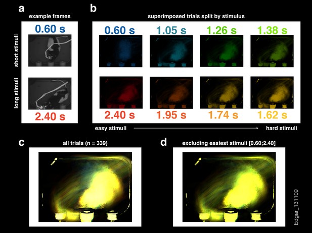
Image frames at the end of the neural analysis window do not show a consistent separation between short and long stimulus trials.
(a) Example frames for a 0.60 and 2.40 s stimulus trials (top and bottom, respectively) at stimulus offset. (b) Superimposed frames (thresholded and background subtracted) for each stimulus type (same color conventions as in Figure 3a). (c) sum of all frames shown in (b). (d) Same as in (c) but excluding the easiest short (0.60 s) and long (2.40 s) stimulus trials. The data show are from the same session presented in Figure 3b.
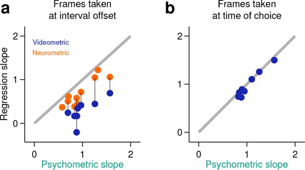
Behavior at the end of the neural analysis window did not explain the categorization performance of neural populations.
(a) Neurometric (orange data points) or videometric (purple data points) logistic slope plotted against the psychometric slope for each session in the upper tercile with respect to simultaneously recorded population size. (b) Videometric slope plotted against the psychometric slope where the videometric curve was built using image frames taken at the time that animals expressed their choice.
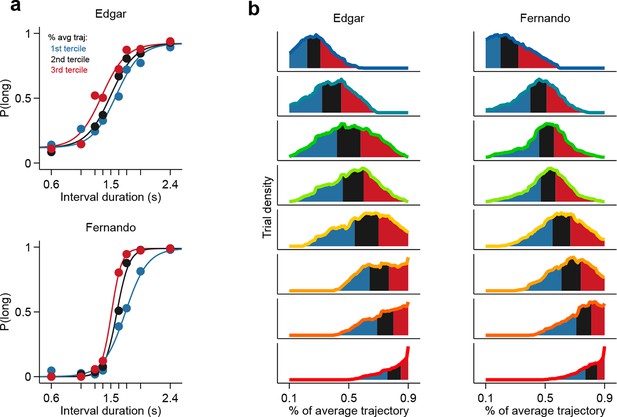
Population state at interval offset can explain behavioral performance.
(a) Psychometric curves constructed from trials separated according to whether the population state at stimulus offset had advanced more or less along the mean trajectory for rats Edgar (top) and Fernando (bottom) (b) Distributions of projection on normalized mean trajectory for all trials for each stimulus are shown for rats Edgar (left) and Fernando (right). The equal area bins shown correspond to the groups of trials used for constructing the three psychometric curves shown in (a).
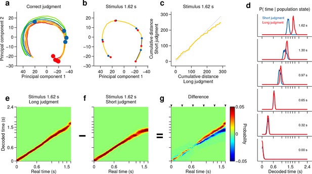
Smoothly changing population state encodes elapsing time in accordance with perceptual report for a long stimulus.
(a) Low dimensional representation of population state during entire interval period of correct trials. Line colors indicate interval duration (warmer colors are longer intervals, as in Figure 3a). Dots are placed at the interval offset end, and their color indicates judgment (blue: short; red: long). (b–g) Population state and decoded time for a single long, near boundary stimulus interval (1.62 s). (b) Yellow curve is same as in (a). Red dots are 6 time points evenly spaced between interval onset and offset. Blue dots are projections of population state during short judgment trials. Grey lines link population states at equivalent time points. (c) Average cumulative distance travelled in full neural space along trajectory represented in (b) on long versus short judgment trials. (d) Posterior probability of time given population state at the time points indicated in (b), averaged within trials of each judgment type. (e,f) Same as (d) for the entire interval period. (g) Difference between posteriors for long and short judgment trials. Arrowheads indicate same time points used in (b,d). n = 433 neurons from 3 rats. See Figure 4—figure supplement 1 for a different near boundary stimulus, and Figure 4—figure supplement 2 for data from individual subjects.
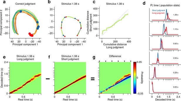
Smoothly changing population state encodes elapsing time in accordance with perceptual report for a short stimulus.
(a) Low dimensional representation of population state during entire interval period of correct trials. Line colors indicate interval duration (same color code as in Figures 3 and 4). Dots are placed at the interval offset end, and their color indicates judgment (blue: short; red: long). (b-g) Population state and decoded time for a single short, near boundary stimulus interval (1.38 s). (b) Green curve is the population state trajectory for long judgment trials. Red dots are 6 time points evenly spaced between interval onset and offset. Blue dots are projections of population state during short judgment trials. Grey lines link population states at equivalent time points. (c) Average cumulative distance travelled in full neural space along trajectory represented in (b) on long versus short judgment trials. (d) Posterior probability of time given population state at the time points indicated in (b), averaged within trials of each judgment type. (e,f) Same as (d) for the entire interval period. (g) Difference between posteriors for long and short judgment trials. Arrowheads indicate same time points used in (b,d).
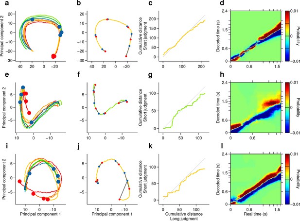
Single subjects show smoothly changing population states that encode elapsing time in accordance with perceptual report.
(a,e,i) Low dimensional representation of population state during entire interval period of correct trials of rats Bertrand (a), Edgar (e) and Fernando (i). Line colors indicate interval duration (warmer colors are longer intervals, as in Figures 3 and 4). Dots are placed at the interval offset end, and their color indicate choice (blue: short; red: long). (b,f,j) Yellow/green line is same as in (a,e,i) for a single near boundary stimulus interval (1.62/1.38 s; stimulus of highest choice variance for each subject). Red dots are 6 time points evenly spaced between interval onset and offset. Blue dots are projections of population state during short judgment trials. Grey lines link population states at equivalent time points. (c,g,k) Average cumulative distance travelled in full neural space along trajectory represented in (b,f,j) on long versus short judgment trials. (d,h,l) Difference between posteriors for long and short judgment trials for rats Bertrand (d), Edgar (h) and Fernando (l).
Videos
Video clips from the entire stimulus period do not show a consistent separation between short and long stimulus trials.
Superimposed video clips (thresholded and background subtracted) for each stimulus type and for the corresponding stimulus duration (same color conventions as in Figure 3a and Figure 3—figure supplement 1). Red stop marks signal the end of each video and the corresponding stimulus duration.


