Active sensing in the categorization of visual patterns
- University of Cambridge, United Kingdom
- Central European University, Hungary
Figures
Figure 1
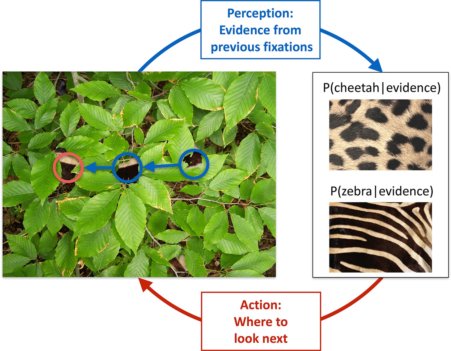
Active sensing involves an interplay between perception and action.
When trying to categorize whether a fur hidden behind foliage (left) belongs to a zebra or a cheetah, evidence from multiple fixations (blue, the visible patches of the fur, and their location in the image) needs to be integrated to generate beliefs about fur category (right, here represented probabilistically, as the posterior probability of the particular animal given the evidence). Given current beliefs, different potential locations in the scene will be expected to have different amounts of informativeness with regard to further distinguishing between the categories, and optimal sensing involves choosing the maximally informative location (red). In the example shown, after the first two fixations (blue) it is ambiguous whether the fur belongs to a zebra or a cheetah, but active sensing chooses a collinearly located revealing position (red) which should be informative and indeed reveals a zebra with high certainty. Note that this is just an illustrative example.
Figure 2 with 1 supplement

Image categorization task and participants’ performance.
(A) Example stimuli for each of the three image types sampled from two-dimensional Gaussian processes. (B) Experimental design. Participants started each trial by fixating the center cross. In the free-scan condition, an aperture of the underlying image was revealed at each fixation location. In the passive condition, revealing locations were chosen by the computer. In both conditions, after a random number of revealings, participants were required to make a category choice (patchy, P, versus stripy, S) and were given feedback. (C) Categorization performance as a function of revealing number for each of the three participants (symbols and error bars: mean SEM across trials), and their average, under the free-scan and passive conditions corresponding to different revealing strategies. Lines and shaded areas show across-trial mean SEM for the ideal observer model. Figure 2—figure supplement 1 shows categorization performance in a control experiment in which no rescanning was allowed.
Figure 2—figure supplement 1

Performance in the no-rescanning control experiment.
Categorization performance as a function of revealing number for participants in the control (no rescanning) and the average participant in the main experiment (rescanning) in which rescanning was allowed (cf. Figure 2C).
Figure 3 with 3 supplements

Density maps of relative revealing locations and their correlations.
(A) Revealing density maps for participants and BAS. Last three columns show mean-corrected revealing densities for each of the three underlying image types (removing the mean density across image types, first column). Bottom: color scales used for all mean densities (left), and for all mean-corrected densities (right). All density maps use the same scale, such that a density of 1 corresponds to the peak mean density across all maps. Figure 3—figure supplement 1 shows revealing density maps obtained for participants in a control experiment in which no rescanning was allowed. Figure 3—figure supplement 2 shows the measured saccadic noise that was incorporated into the BAS simulations. Figure 3—figure supplement 3 shows density maps separately for correct and incorrect trials. (B) The curves are correlations for individual participants as a function of revealing number with their own maps (left) and the maps generated by BAS (right). The bars are correlations at 25 revealing (see Materials and methods). Orange shows within image type correlation, ie. correlation between revealing densities obtained for images of the same type, and purple shows across image type correlation. Data are represented as mean SD for the curves and mean 95% confidence intervals for the bars.
Figure 3—figure supplement 1
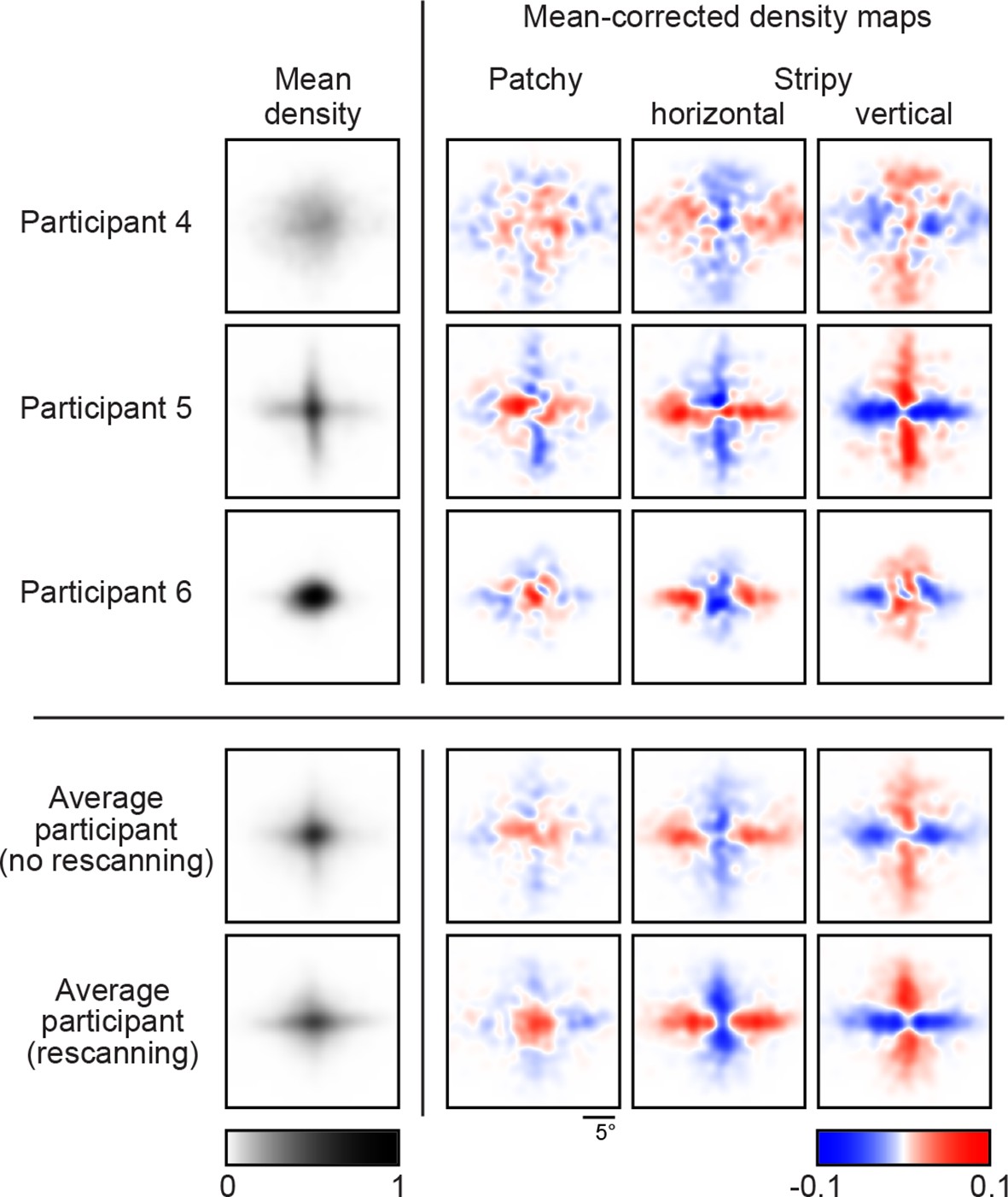
Revealing density maps in the no-rescanning control experiment.
Revealing density maps in the control (no rescanning) and the average participant in the main experiment (rescanning) in which rescanning was allowed (cf. Figure 3A).
Figure 3—figure supplement 2
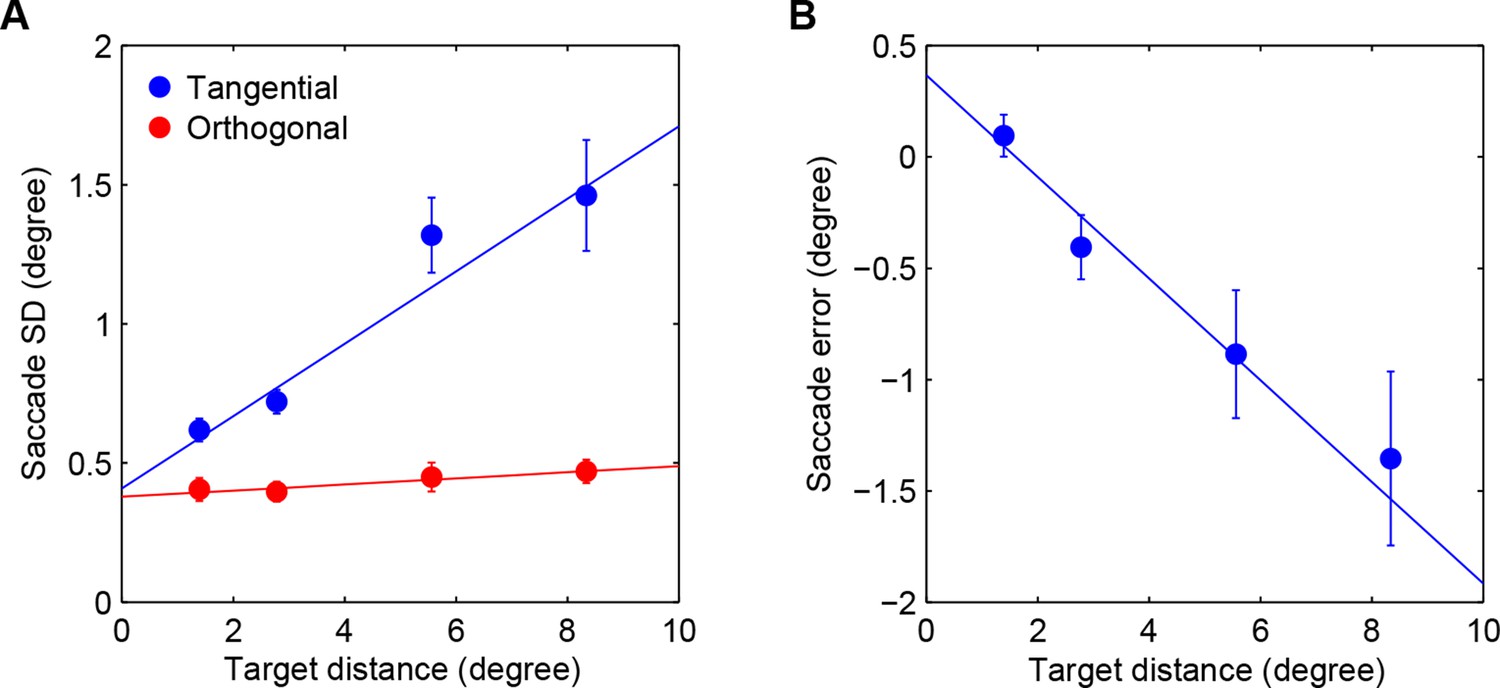
Saccadic variability and bias.
(A) Saccadic standard deviation both along (tangential) and orthogonal to the target direction with linear regression giving SD = 0:13×distance+0:41° and 0:011 distance+0:38°, respectively. (B) Saccadic bias along the target direction (negative is undershoot) with linear regression giving bias = 0:23×distance+0:37°. Error bars are SEM across participants.
Figure 3—figure supplement 3
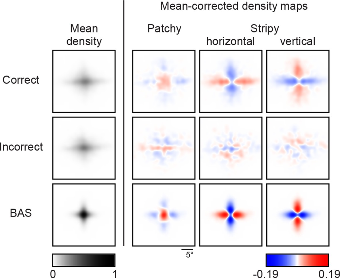
Revealing density maps of the average participant in the main experiment split into correct and incorrect trials, and the BAS revealing maps.
https://doi.org/10.7554/eLife.12215.009
Figure 4 with 1 supplement
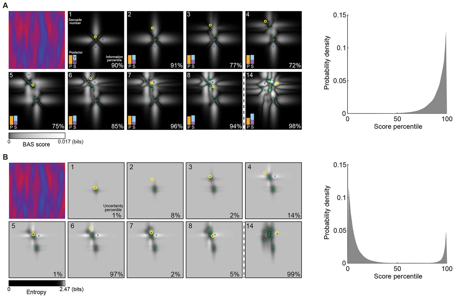
Example trial of the Bayesian active sensor (BAS) and its maximum entropy variant.
(A) The operation of BAS in a representative trial for saccades 1–8 and 14 (underlying image shown top left). For each fixation (left, panels), BAS computes a score across the image (gray scale, Equation 1). This indicates the expected informativeness of each putative fixation location based on its current belief about the image type, expressed as a posterior distribution (inset, lower left), which in turn is updated at each fixation by incorporating the new observation of the pixel value at that fixated location. Crosses show the fixation locations with maximal score for each saccade, green dots show past fixation locations chosen by the participant and yellow circle shows current fixation location. Percentage values (bottom right) show their information percentile values (the percentage of putative fixation locations with lower BAS scores than the one chosen by the participant). Histogram on the right shows distribution of percentile values across all participants, trials and fixations. (B) Predictions of the maximum entropy variant (the first term in Equation 1) as in (A). For saccades 1–3, the fixation locations with maximal score (crosses) are not shown because the maxima comprise a continuous region near the edge of the image instead of discrete points. Note that entropy can be maximal further (eg. fixation 4) or nearer the edges of the image (eg. fixation 1), depending on the tradeoff between the two additive components defining it: the BAS score, which tends to be higher near revealing locations (panel A), and uncertainty due to the stochasticity of the stimulus and perception noise, which tends to be greater away from revealing locations. Figure 4—figure supplement 1 shows two illustrative examples for this trade-off.
Figure 4—figure supplement 1
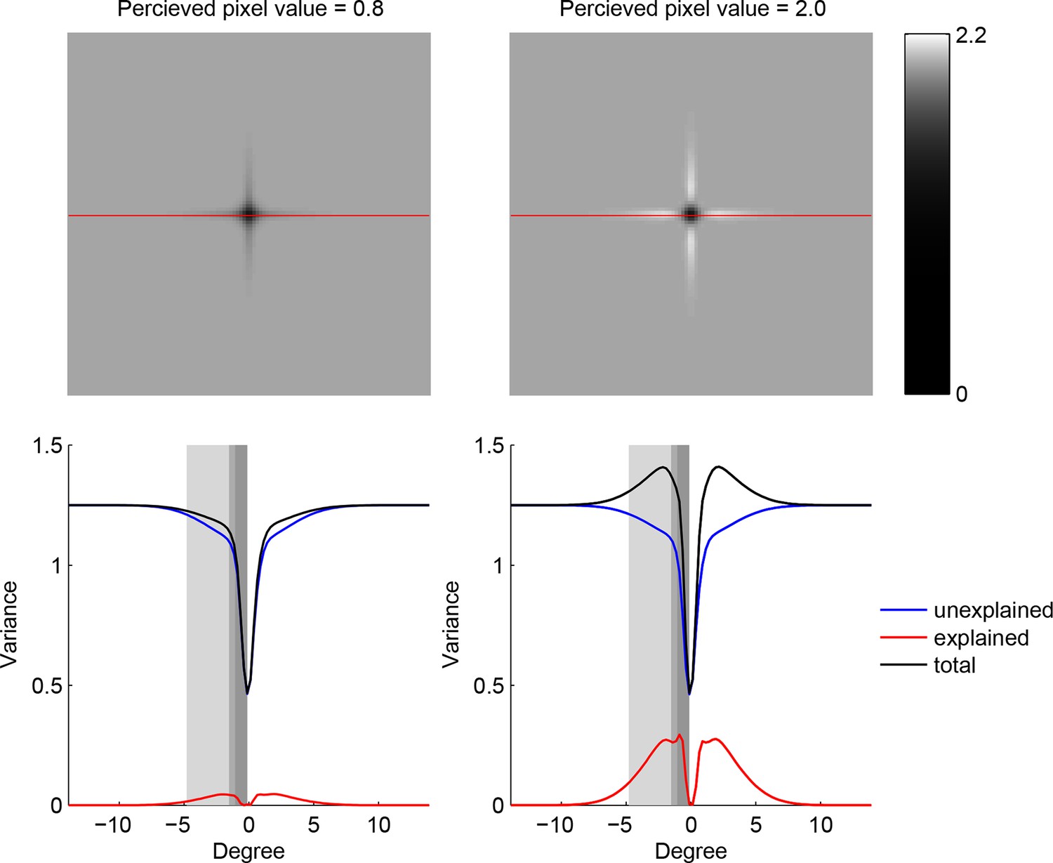
Trade-off between the two components making up total uncertainty underlying the maximum-entropy algorithm.
Top row shows entropy (in bits) of the predictive distributions, , for a grid of locations after one observation. Bottom row shows the corresponding variance decomposition (cf. Equation 1), unexplained (blue) corresponds to “noise” entropy, , explained (red) correspond to the BAS score, Score, and total (black) coresponds to total uncertainty, . The widths of the gray regions correspond to the three length scales with which the three image types are constructed.
Figure 5 with 1 supplement

Information gain as a function of revealing number for different strategies.
(A) Cumulative information gain of an ideal observer (matched to participants’ prior bias and perceptual noise) with different revealing strategies (black, green, and blue) and participants’ own revealings (red). Data are represented as mean SEM across trials. Figure 5—figure supplement 1 shows a measure of efficiency extracted from these information curves across sessions. (B) Information gains for three heuristic strategies (See text for details, and Materials and methods): posterior-independent & order-dependent fixations (orange), posterior-dependent & order-independent fixations (purple), and posterior- & order-dependent fixations (brown). The information gain curves for the three heuristics overlap in all cases. Participants’ active revealings (red lines, as in A) were 1.81 (95% CI, 1.68–1.94), 1.85 (95% CI, 1.72–1.99), and 1.92 (95% CI, 1.74–2.04) times more efficient in gathering information than these heuristics, respectively. Data are represented as mean SEM across trials.
Figure 5—figure supplement 1
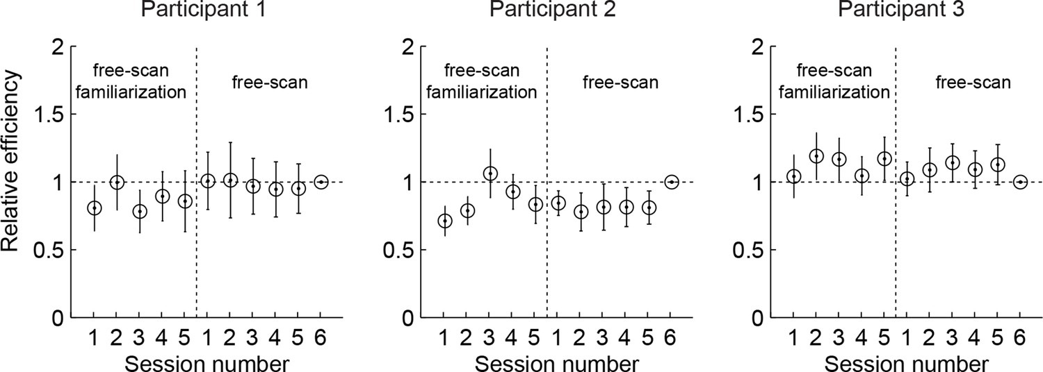
Relative efficiency across free-scan sessions.
Relative efficiency computed as the ratio of the scale parameter as (see Materials and methods) of each session to that of the last session. Circles and lines show mean and SD obtained by bootstrapping trials within a session 50 times. The revealings on day 2-3 (free-scan sessions) were 0.90–1.04 (across participants) times as efficient compared to day 1 revealings (free-scan familiarization sessions). This suggests that participants were already choosing revealing locations on day 1 with near-asymptotic efficiency.
Author response image 1
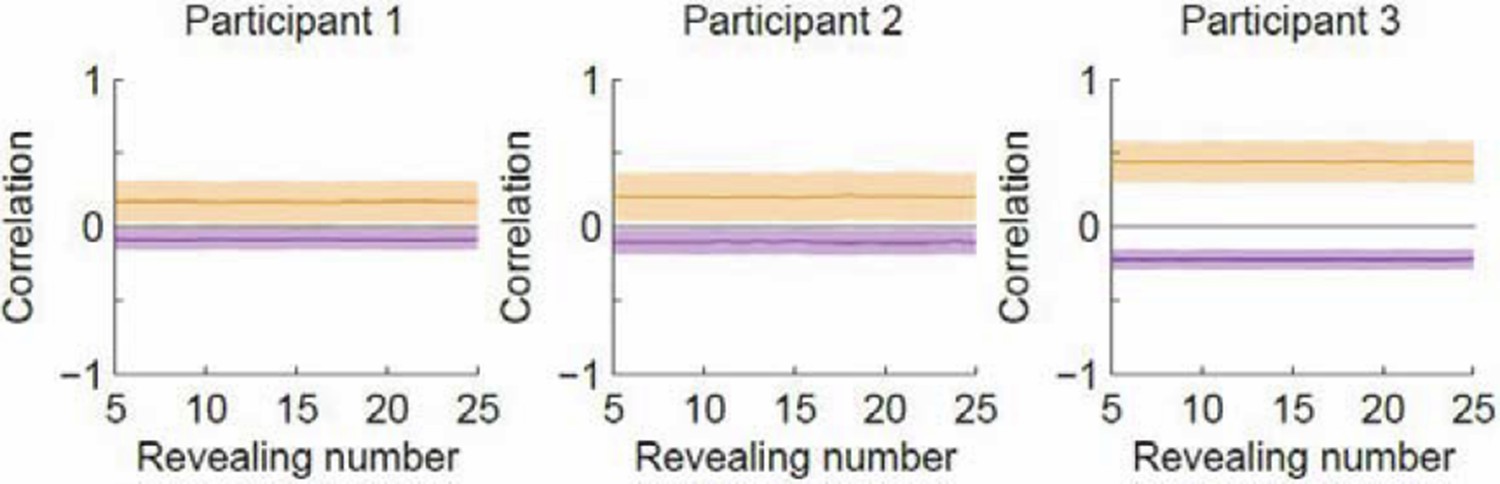
Correlation as a function of revealing number with the revealing number shuffled.
Orange denotes within-type correlation; purple denotes across-type (cf. Figure 3B in the manuscript). Line and shaded area represent mean and SD, respectively.
Author response image 2
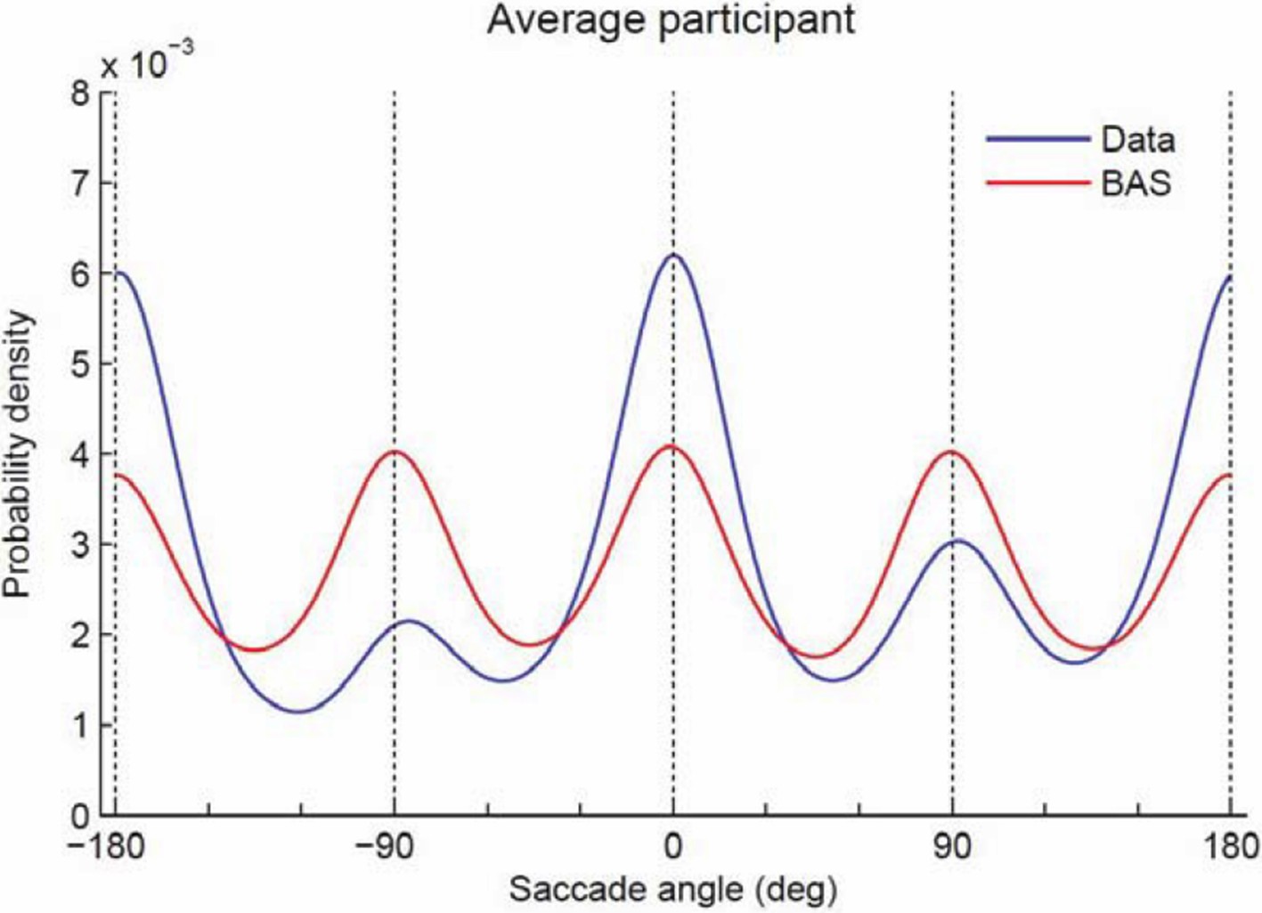
Probability density of saccade angles.
https://doi.org/10.7554/eLife.12215.017Tables
Table 1
Maximum likelihood parameters of the model (see Materials and methods for details) with the best BIC score (see Table 2).
| Participant | Perception noise, σp | Prior bias, Δ | Decision noise | |
|---|---|---|---|---|
| Stimulus-dependent, β | Stimulus-independent, κ | |||
| 1 | 0.5 | 0.58° | 1.4 | 0.044 |
| 2 | 0.5 | 0.61° | 1.9 | 0.12 |
| 3 | 0.3 | 0.54° | 1.5 | 0.10 |
Table 2
Model comparison results using Bayesian information criterion (BIC, lower is better). Each row is a different model using a different combination of included (+) and excluded (–) parameters (columns, see Materials and methods for details). Last column shows BIC score relative to the BIC of the best model (number 4).
| Model | Perception noise, σp | Prior bias | Decision noise | BIC | ||
|---|---|---|---|---|---|---|
| Scale, α | Offset, Δ | Stimulus-dependent, β | Stimulus-independent, κ | |||
| 1 | + | – | – | + | – | 160 |
| 2 | + | – | – | + | + | 139 |
| 3 | + | – | + | + | – | 58 |
| 4 | + | – | + | + | + | 0 |
| 5 | + | + | – | + | – | 105 |
| 6 | + | + | – | + | + | 102 |
Download links
A two-part list of links to download the article, or parts of the article, in various formats.
Downloads (link to download the article as PDF)
Open citations (links to open the citations from this article in various online reference manager services)
Cite this article (links to download the citations from this article in formats compatible with various reference manager tools)
Active sensing in the categorization of visual patterns
eLife 5:e12215.
https://doi.org/10.7554/eLife.12215


