Hippocampal ensemble dynamics timestamp events in long-term memory
Figures
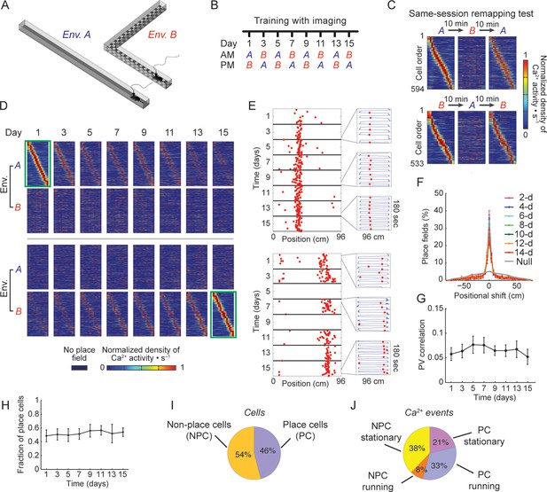
Stable spatial remapping between two familiar environments despite evolving place codes.
(A) Mice trained to run back and forth and collect a liquid reward in two different linear tracks. (B) Experimental timeline. After a pre-training period, we trained and imaged mice in the two environments every two days for 15 days. Each session (AM and PM) consisted of five 3-min trials. (C) Remapping tests within the same session performed on day 16 (top panels) and day 17 (bottom panels) confirmed that CA1 representations of the two environments were different. The test consisted of two trials in one environment followed by three trials in the other environment, and then an additional three trials in the first environment (A→B→A, or B→A→B). Shown are place-field maps ordered according to the place field centroid position in the first two trials of the session in environment A (top) and environment B (bottom). (D) Place field maps for the same cells on multiple days of the experiment, ordered by the place fields’ centroid positions in environment A on day 1 (green frame, top panels), or by the place fields’ centroid positions in environment B on day 15 (green frame, bottom panels). The maps depict the changes in place cell activity patterns in different environments and on different days. (E,F) Place cells that were active on more than one day typically retained their place fields in subsequent sessions. (E) Examples of a place cell active on all days of the experiment in environment B (top), and a place cell active on some days of the experiment in environment A (bottom). Red dots indicate the location of the mouse along the track during cellular Ca2+ excitation. Insets depict the mouse’s trajectory (blue line) and location (red dots) during cellular Ca2+ excitation in individual 3-min trials taken from different days. (F) The distributions of centroid shifts (color indicates the interval between sessions, averaged over five mice, mean ± s.e.m) were, centered at zero, and distinct from the null hypothesis that place cells would randomly alter their place fields (Kolmogorov-Smirnov test, p < 10-14 for all distributions). (G) Average correlations of place cell firing patterns (i.e. the ‘population vector’, PV) during running epochs at different locations along the two linear tracks were low and did not change over time (One-way repeated-measures ANOVA; F<1, p = 0.44). (H) The fraction of place cells out of the population of cells active in both environments on each day also remained stable over time (One-way repeated-measures ANOVA, F(2.18, 8.71) = 1.97, p = 0.19). (I) Average fractions of place cells and non-place cells, and (J) average fractions of Ca2+ events generated by place cells and non-place cells when mice were running or stationary.
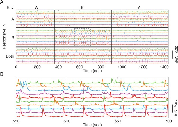
CA1 neurons exhibit selective Ca2+ responses in the two environments.
(A) Example time traces of 30 cells from one mouse, taken from the same-session remapping test. We found cells that responded mostly in environment A (10 cells whose traces are depicted at the top), mostly in environment B (10 cells whose traces are depicted at the middle), or in both environments (10 cells depicted at the bottom). (B) Inset of boxed area in A.
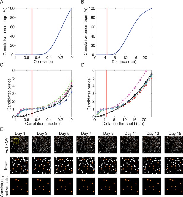
Accurate across-session cell identification based on correlation or distance between candidate cells.
(A–D) We followed and revalidated a previously established routine for across-session cell identification (Ziv et al., 2013). For each session we created a map containing the spatial filters of all cells that were active in that session. We cross-registered the maps from different sessions using one session as a reference. We then analyzed the correlations and distances between neighboring cells in each session, using these distributions to threshold the acceptance of candidate cells as the same. (A) Cumulative percentage of nearest neighbors as a function of their spatial correlation within a session. The red dashed line, set at correlation = 0.7, represents the threshold for a candidate cell to register as the same neuron across sessions. Correlations with nearest neighbors were always < 0.6 within-sessions. We chose a higher threshold of 0.7 for registration of cells across sessions to further reduce the likelihood of incorrectly registering different cells as the same neuron. (B) Cumulative percentage of nearest neighbors as a function of centroid distance within a session. The red dashed line, set at distance = 5 μm, represents the threshold for a candidate cell to register as the same neuron across sessions. Nearest neighbors’ centroids distances were always > 6 μm within a session. We chose a lower threshold of 5 μm for registration of cells across sessions to further reduce the likelihood of incorrectly registering different cells as the same neuron. (C) Average number of candidates per cell to register as the same neuron as a function of the spatial correlation threshold. Colored dashed curves represent the data obtained from five mice over 16 sessions in the two environments. The black solid curve represents shuffled data obtained by performing cell registration on mixed sessions from different mice. The number of candidates increases monotonically as the correlation threshold is lowered. At high correlation thresholds > 0.85, the number of candidates quickly grows mostly due to cells that are actually the same neuron. At low correlation thresholds < 0.5, the number of candidates quickly grows mostly because of cells that are not the same neuron. As expected for an accurate cell registration, in the intermediate range, the number of candidates is maintained at approximately 1 per cell. Thus, the registration of cells across sessions is insensitive to the exact choice of the correlation threshold in the range of 0.5-0.85. Note that there is no such threshold regime for the shuffled data. (D) Average number of candidates per cell to register as the same neuron as a function of the centroid distance threshold. Colored dashed curves represent data obtained from 5 mice over 16 sessions in the two environments. The black solid curve represents shuffled data obtained by performing cell registration on mixed sessions from different mice. The number of candidates increases monotonically as the distance threshold is raised. At small distance thresholds < 3 μm, the number of candidates quickly grows mostly because of cells which are indeed the same neuron. At large distance thresholds > 8 μm, the number of candidates quickly grows mostly due to cells that are not the same neuron. As expected for an accurate cell registration, in the intermediate range, the number of candidates is maintained at approximately 1 per cell. Thus, the registration of cells across sessions is insensitive to the exact choice of the centroid distance threshold in the range of 3–8 μm. Note that there is no such threshold regime for the shuffled data. (E) Projection of all spatial filters onto a single map obtained independently from eight separate sessions in the same environment. The top row shows the entire field of view and the middle and bottom rows show only the partial field of view marked by the inset. Cells that were registered as the same neuron in all sessions (threshold correlation = 0.7) are colored orange, whereas the rest are colored white. Images at the bottom row indicate that the spatial filters for this subset were consistent in their shape and location across sessions.
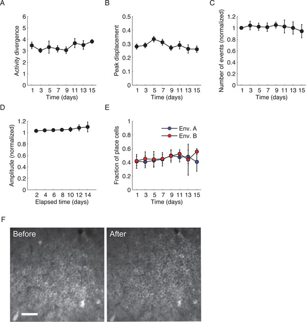
Stable neuronal function and environment-specific activity.
(A,B) Both ‘activity divergence’, the difference in event rate between trials in different environments relative to the difference in event rate between trials in the same environment (A), and ‘peak displacement’, the average distance between locations of peak activity in different environments (B), did not change over the course of the experiment (One-way repeated-measures ANOVA; F(1.9, 7.6) = 1.06, p = 0.39 and F(2.6, 10.5) = 1.22, p = 0.345 respectively). (C) Average number of Ca2+ events detected on different days of the experiment did not change with time (One-way repeated-measures; F(1.87, 7.49) = 1.19, p = 0.35). (D) Amplitudes of Ca2+ events remained similar over the course of the experiment (One-way repeated-measures; F(1.32, 5.29) = 3.29, p = 0.35.). (E) Fractions of place cells from the population of cells active in each environment were similar for both environments and did not change with time. Two-way repeated measures ANOVA between environment A and B (F < 1, p = 0.42), over time (F(2.32,9.30) = 1.99, p = 0.19), and environment X time interaction (F(1.93, 7.72) = 1.71, p = 0.243). Data are mean ± s.e.m. (F) Representative two-photon microendoscopy images of CA1 neurons performed before and after the experiment. The images revealed no increase in the number of cells with filled nuclei (a marker for GCaMP-induced neuronal morbidity). Scale bar is 50 μm.
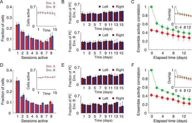
Activity and long-term dynamics of GCaMP6s- and GCaMP6f expressing cells.
(A,D) Distribution of the total number of sessions in which cells were active for GCaMP6s (A) and GCaMP6f (D) (n=3, and n=2, respectively). Inset, the fraction of active cells detected in each session (red – environment A, blue – environment B). (B,E) Fraction of cells with significant place fields, expressed as the fraction of cells found in each session for each motion direction (top - environment A, bottom - environment B) for GCaMP6s (B) and GCaMP6f (E). (C,F) Correlations between cell activity patterns within the same environment (green data) or between different environments (red data) for GCaMP6s (C) and GCaMP6f (F). Ensemble activity correlations decay with elapsed time. Inset, the probability that a cell active on one day will be active on subsequent days in the same environment (green data) or in a different environment (red data). The recruitment probability decayed with elapsed time. Data are mean ± s.e.m.
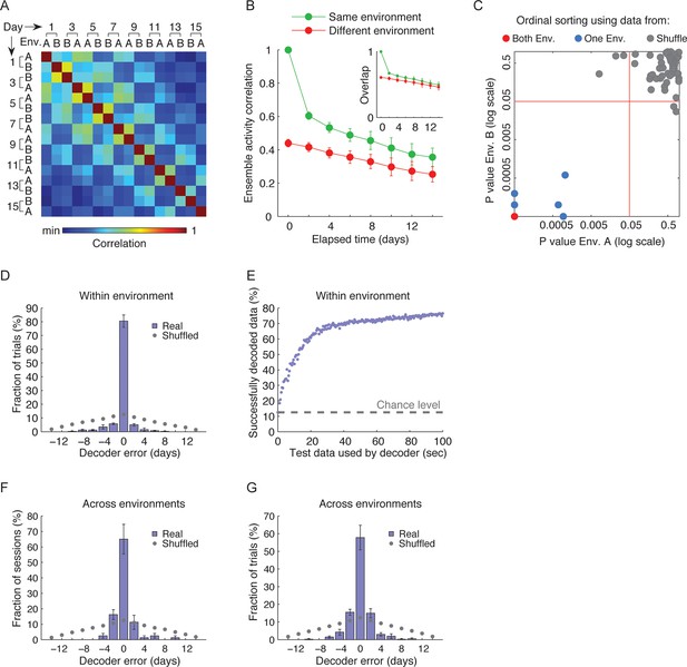
CA1 ensemble codes are informative about the temporal relationship between experienced events.
(A) Pairwise correlations between the complete activity patterns of all cells in different environments and different days (an average of n = 5 mice). The checkerboard pattern reveals the resemblance between the episodic representations of the same environments at different times. (B) Correlations between cell activity patterns within the same environment (green) or between different environments (red) decay with time. This trend is also visible in A when considering the changes in correlations along a row. Inset, the probability that a cell active on one day will be active on subsequent days in the same environment (green) or in a different environment (red) decayed with time (mean ± s.e.m). (C) Performance of the ordinal time decoder. Red dots indicate perfect performance, as was achieved by using data from both environments together (see Figure 2—figure supplement 2). Sorting of the sessions using data from one of the environments was highly significant in comparison with the results obtained using data in which the day labels of each cell’s activity patterns were randomly shuffled (gray dots, n =10 shuffles per mouse). Red lines indicate p = 0.05. (D,E) A ‘within-environment time decoder’ was trained and tested on data from the same environment. (D) Distributions of the decoder’s errors in inferring the day from which the test data (single trials) were taken. The decoder successfully inferred the day from which the test data was taken in the majority of cases, but performed at chance level on shuffled data (gray dots, shuffled data as in C). (E) Successful time decoding (decoder error = 0 days) depended on the amount of test data used by the decoder. Shown are percentages of accurate decoding for test data of different durations. Performance using test data segments as short as 1 sec exceeded chance level (12.5%, gray horizontal line). (F,G) An ‘across-environments time decoder’ was trained on data from one environment (A or B) and tested on data from the other environment (B or A, respectively). (F) Distributions of the decoder’s errors in inferring the day from which a test data consisting of single sessions (F) or single trials (G) were taken. The decoder successfully inferred the day from which the test data was taken in the majority of cases, but performed at chance level on shuffled data (shuffled data as in C). Data in B and D-G are mean ± s.e.m.
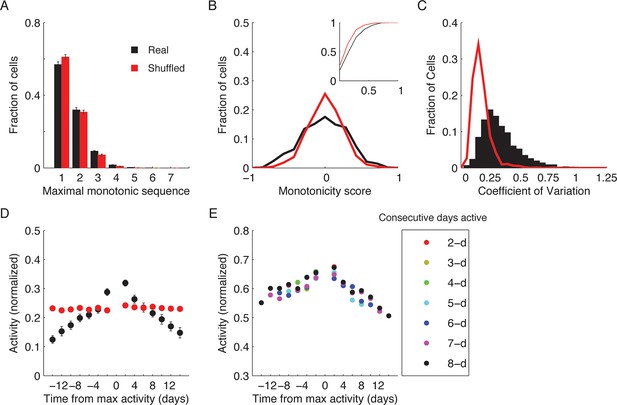
Within-environment cell-level dynamics (A–E).
(A) Distribution of maximal monotonic sequence length for all cells (black) and for the shuffled data (red). None of the cells exhibited monotonic changes in event rates throughout the experiment (0.7% of cells with a monotonic sequence-length ≥ 4). However, the single-cell dynamics were slightly more monotonic than shuffled data (average maximal sequence length is 1.56 for real data and 1.48 for shuffled data). Data are mean ± s.e.m. (B) Distribution of the monotonicity score. Inset, cumulative distribution of the absolute values of the score for all cells. In the real data (black) there were more strongly increasing and decreasing cells than in the shuffled data (red) suggesting that cell-level changes in event rates are time dependent and are not purely due to noise (Kolmogorov-Smirnov test, p < 10−10). (C) Distribution of event rates’ coefficient of variation (CV) for the cells that were active in all sessions (black) and the CV distribution of a population of simulated cells with equivalent average event rates that follow a stationary Poisson model of activity (red). Note that cells exhibit higher CV than Poisson distribution (median CV is 0.30 for real data and 0.16 for the equivalent Poisson model) indicating that even cells that were active in all days of the experiment do not preserve their firing rates over days. (D,E) Gradual ensemble dynamics emerges when averaging the activity over the entire population. (D) Normalized event rate aligned to the day of peak event rate, averaged over all cells. The real data (black) shows a clear relationship between the ensemble average event rate and time difference from the session with the maximal event rate. Data are mean ± s.e.m. Shuffled data shown in red. (E) Same as in D for subgroups of different maximal consecutive activity segment lengths (2–8 days, maximal-length active segment is shown). Thus, the trend shown in D is not only due to the recruitment dynamics but also due to gradual changes in event rates of active cells.
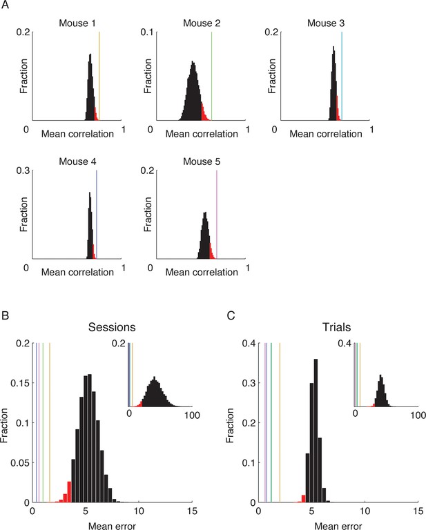
Time decoders accurately expose temporal information in all individual mice.
(A) Distributions of the correlations between ensemble activity patterns averaged over the seven pairs of neighboring days for all 8!/2 possible day permutations (the top 5% of the correlations values are colored red). Colored vertical lines indicate the mean correlations between activity patterns of pairs of neighboring days (taken from both environments together) from the actual data. In all mice, the actual data yielded the highest mean correlation of all possible permutations. Therefore, maximizing the mean correlation between pairs of days allows for an accurate ordering of the data from different days of the experiment (p < 5 · 10−5 for each mouse). (B,C) Performance of across environment time decoder on whole sessions (B) and single trials (C) exceeded the chance level in all mice. (B) Distribution of mean errors over all 16 sessions for random day labeling of each session (n = 100,000). The top 5% of the performances are colored red and represent a significantly small mean error. Colored vertical lines represent the mean error for each mouse (color code as in A; p < 5 · 10−5). Inset, distribution of mean squared error (MSE) of chance levels and individual mouse performances (vertical lines). (C) Distribution of mean errors over all 80 trials for random day labeling of each trial (n = 100,000). The top 5% of the performances are colored red and represent a significantly small error. Colored vertical lines represent the mean error for each mouse (color code as in A; p < 5 · 10−5 for each mouse). Inset, distribution of mean squared error (MSE) of chance levels and individual mouse performances (vertical lines).
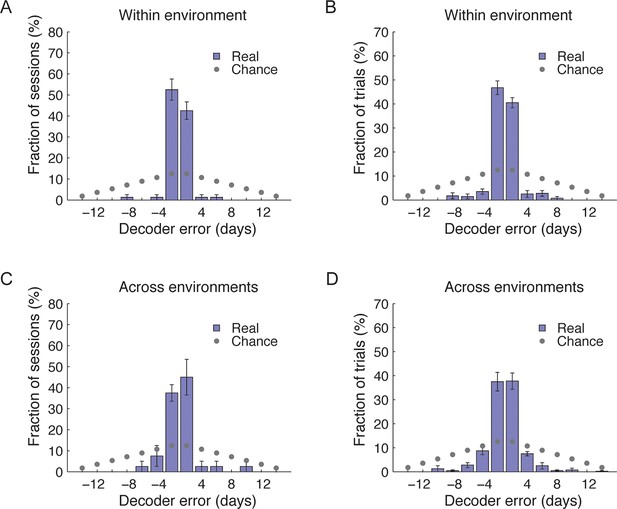
Time decoders accurately infer the time of the episode even when the tested session is excluded from the training data (A–D).
(A,B) Distributions of the decoders’ errors in inferring the day from which the test sessions (A) or trials (B) were taken within environment. The decoder inferred either the recording day before or after the day the test data was taken from in 95% of the sessions and 87.25% of the trials, significantly higher than chance levels (gray dots). (C,D) Distributions of the decoders’ errors in inferring the day from which the test sessions (C) or trials (D) were taken across-environments. The decoder inferred either the recording day before or after the day the test data was taken from in 82.5% of the sessions and 75.25% of the trials, significantly higher than chance levels (gray dots). (z-test, p < 6 · 10−7 for all comparisons). Data are mean ± s.e.m.
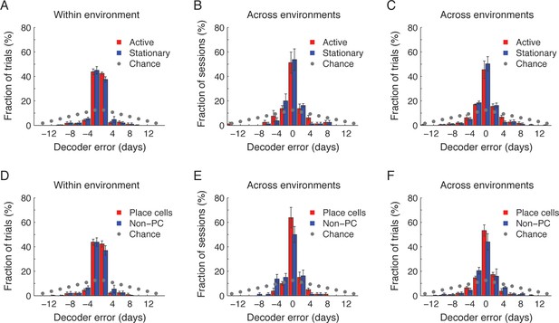
CA1 ensemble place codes and non-place codes are informative about the temporal relationship between experienced events.
To quantify whether non-place codes contained temporal information we analyzed the performance of the different time decoders, separately for periods in which the mouse was active versus stationary (A–C) and for place cells versus non-place cells (D–F). Active periods were defined as times when the animal was at velocity ≥1 cm/sec and located more than 8cm from either ends of the track. Place cells were defined as cells with significant place coding in at least one session. (A,D) Distributions of the time decoders’ errors in inferring the day from which the test trials were taken within environment (as in Figure 2— figure supplement 3B the tested session was excluded from the training data), for active periods versus stationary periods (A; paired t-test, p >0.36) and for place cells versus non-place cells (D; paired t-test, p >0.27). (B,E) Distributions of the time decoders’ errors in inferring the day from which the test sessions were taken across environment, for active periods versus stationary periods (B; paired t-test, p >0.81) and for place cells versus non-place cells (E; paired t-test, p >0.14). (C,F) Distributions of the time decoders’ errors in inferring the day from which the test trials were taken across environments, for active periods versus stationary periods (C; paired t-test, p >0.25) and for place cells versus non-place cells (F; paired t-test, p >0.19). All data in A-F is significantly different than chance (paired t-test, p <10-6 for all comparisons).
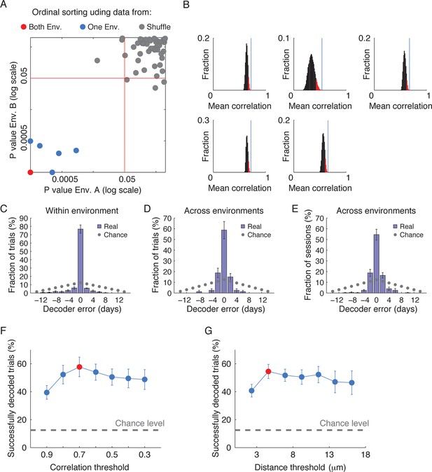
Time decoding is robust to changes in the across-session cell identification method.
(A–D) We re-analyzed the data using the alternative, distance-based across-session cell identification routine, with a threshold distance of 5μm (See Figure 1—figure supplement 2). Using this alternatively analyzed data, we performed the same time decoding analyses shown in Figure 2D–H. (A) Performance of the ordinal time decoder. The red dots indicate perfect performance, as was achieved by using data from both environments together. Sorting of the sessions using data from one of the environments significantly outperformed sorting of the sessions using data in which the day labels of each cell’s activity patterns were randomly shuffled (gray dots, n =10 shuffles per mouse). (B) Distributions of the correlations between ensemble activity patterns averaged over the seven pairs of neighboring days for all 8!/2 possible day permutations. Vertical lines indicate the mean correlations between activity patterns of pairs of neighboring days of the actual data. As in the analysis shown in Figure 2C and Figure 2—figure supplement 2A, we found that in all mice, actual data yielded the highest mean correlation of all possible permutations. (C) A ‘within-environment time decoder’ was trained and tested on data from the same environment. Shown are distributions of the decoder’s errors in inferring the day from which a test data (single trials) was taken. The decoder successfully inferred the days from which the test data was taken in the majority of cases. (D,E) An ‘across-environment time decoder’ was trained on data from one environment (A or B) and tested on data from the other environment (B or A, respectively). Shown are distributions of the decoder’s errors in inferring the day from which a test data consisting of single sessions (D) or single trials (E) were taken. The decoder successfully inferred the day from which the test data was taken in the majority of cases. (F, G) Changing the threshold for a candidate cell to register as the same neuron across sessions did not alter the conclusions regarding the performance of the across environment time decoder. (F) The success rates of the time decoder changed only slightly and were highly significant in comparison to the chance level over a broad range of thresholds used by the correlation-based across-session cell identification routine (z-test, p < 10-8 for all comparisons). The red data point indicates optimal threshold, consistent with an independent analysis shown in Figure 1—figure supplement 2C. (G) The success rates of the time decoder changed only slightly and were highly significant in comparison to the chance level over a broad range of thresholds used by the distance-based across-session cell identification routine (z-test, p < 10-8 for all comparisons). The red data point indicates optimal threshold, consistent with an independent analysis shown in Figure 1—figure supplement 2D. Data are mean ± s.e.m.
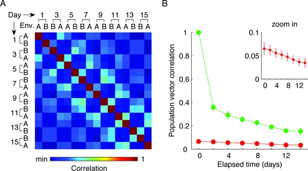
The two environments can be distinguished according to CA1 place cell firing patterns regardless of recording day (A,B).
(A) Average pairwise correlations of firing patterns (i.e. the ‘population vector’, PV, of all place cells) at different environments and different days (an average of n = 5 mice). The checkerboard pattern reveals the resemblance between the episodic representations of the same environments at different times. (B) PV correlations within the same environment (green data) or between different environments (red data) as a function of elapsed time. Although PV correlations decay as a function of elapsed time, within environment PV correlations from sessions that are two weeks apart remain higher than across-environment PV correlations from the same day. Inset, zoom in on the low PV correlation values (mean ± s.e.m).


