RETRACTED: A mathematical model explains saturating axon guidance responses to molecular gradients
- The University of Queensland, Australia
- University College London, United Kingdom
Figures
Figure 1

Model set-up and the noiseless case.
(A) The axon starts growing from the soma (black segment) at initiation angle ϕ(0). At each time point, the bearing is θ(t), and the bearing change between t and t + 1 is Δθ(). ϕ() is the angle of the vector connecting the current position of the growth cone with the anchor point. Ψ is the fixed gradient direction. (B) The turning angle ψturn at time is the angle between the initial direction of growth, and the line joining the initial and current positions of the growth cone. (C) Simulation of the growth cone angle using Equation (1) in the noiseless case (ξ = 0) with the same = 1 and different values of b. The dashed line is the power law . In the long time limit, this law accurately describes the angle of the growth cone. (D) Simulations of the trajectories for different combinations of and in the absence of noise. Larger leads to stronger turning. When = 0, the growth cone very rapidly aligns with the gradient. The persistence term ( > 0) leads to incomplete turning.
-
Figure 1—source code 1
The code to simulate the trajectories based on Equation 1 in the noiseless case.
- https://doi.org/10.7554/eLife.12248.005
Figure 2
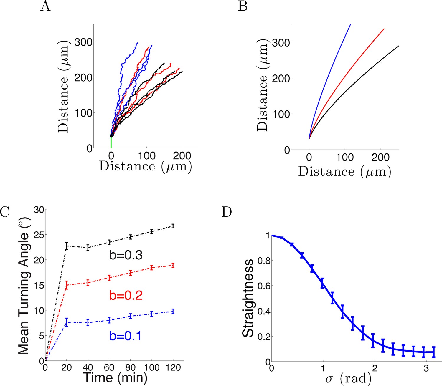
Model results with noise.
(A) Long-term behavior of growth cones: Simulation of 9 axons with fixed growth rate and noise in bearing changes (ξ ∼ N(0, π/4) radians) starting at ϕ(0) = 90° subject to the gradient direction Ψ = 0 with persistence = 1 and bias = 0.1 (blue), = 0.2 (red) and = 0.3 (black) after 150 steps (12.5 hr of real time). (B) The trajectories with the same parameters without noise. (C) The turning angles over time (mean ± SEM) of 1000 axons for different values of (0.1,0.2, 0.3) and = 1. (D) Straightness (mean ± std) decreases as the noise variance increases.
-
Figure 2—source code 1
The code to simulate the trajectories based on Equation 1 in the noisy case.
- https://doi.org/10.7554/eLife.12248.007
Figure 3
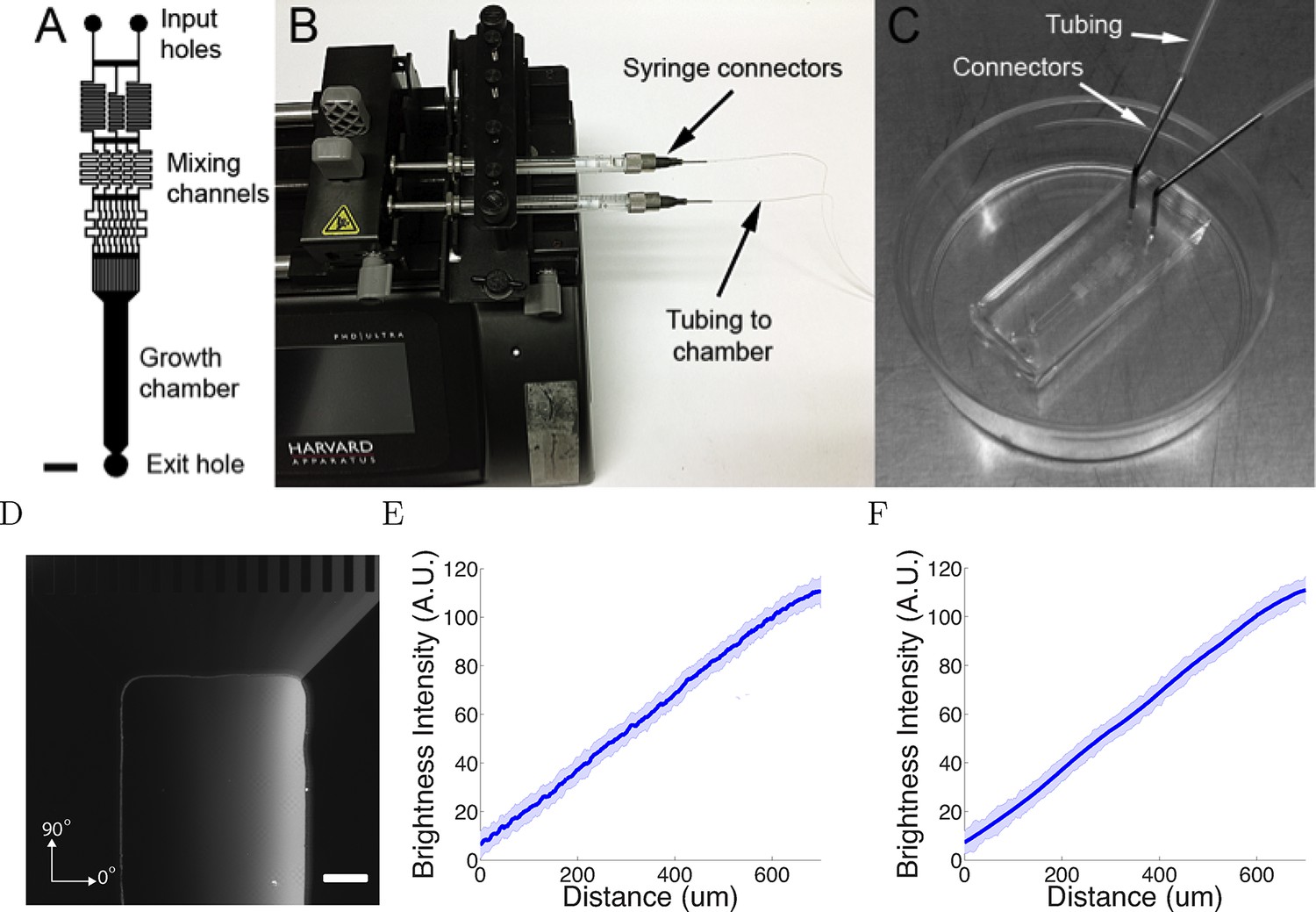
The microfluidic assay.
(A) The design of the chamber: the two solutions were pumped into the inlets and mix in the mixing channels before flowing into the growth chamber where the cells are plated. The mixing channels were of height 50 μm and width 50 μm. Scale bar 1 mm. (B, C) Photo of the experimental setup: two glass syringes attached to a Harvard pump injected the solutions into the chamber bonded on a 35 mm plastic plate. (D) Two solutions, one of which contained 0.1% (v/v) dextran fluorescently labelled with tetramethylrhodamine, were used to visualize the gradient. Brighter regions indicate higher concentrations. Scale bar 200 μm. (E, F) Line-scan measurements of fluorescence intensity across the device show a linear gradient which persists for at least 20 hr ( = 0h (E) and = 20h (F) ). The shaded errorbars show standard deviations across 10 chambers.
-
Figure 3—source data 1
The average brightness intensity and noise in the microfluidic chamber at 0 and 20 hr.
The average and noise were estimated from 5 min interval timelapse imaging over an 1-hr period.
- https://doi.org/10.7554/eLife.12248.009
Figure 4
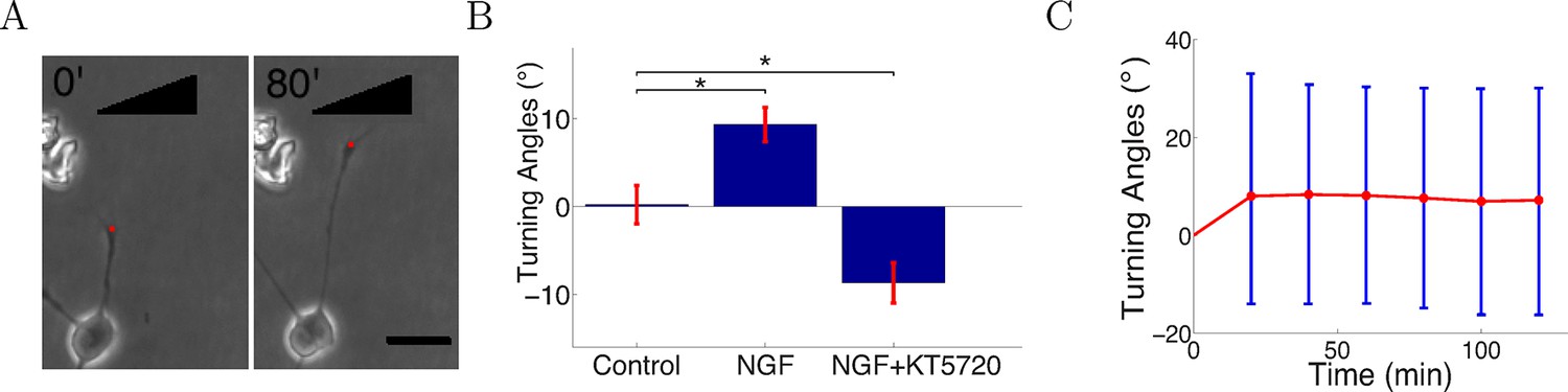
Turning in microfluidic gradients.
(A) Images of a representative axon initially almost perpendicular to the gradient at the beginning and end of the measurement after 80 min. Scale bar 20 μm. The red dots are the positions of the growth cone. (B) Summary of turning angles in the three conditions (mean ± SEM): control 0.2 ± 2.1° (n=120), NGF gradient (0–10 nM) 9.3 ± 1.9° (n=143), NGF gradient (0–10 nM) + KT5720−8.8 ± 2.2° (n=112). *: p < 0.01 t-test in both cases. (C) The means (red) and standard deviations (blue) of turning angles of 143 axons over time for the attractive case.
-
Figure 4—source data 1
The turning angles at different time points from the start of the experiment.
- https://doi.org/10.7554/eLife.12248.011
Figure 5
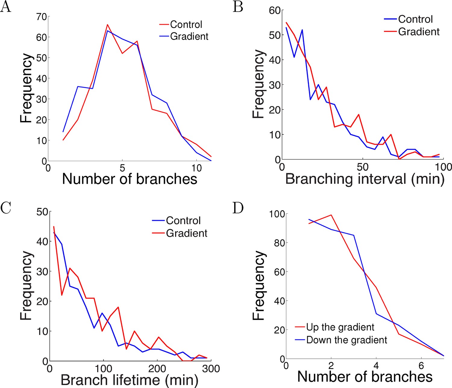
The gradient did not affect branch extension and retraction rates.
(A) Histogram of the number of cells with different numbers of branches after 5 hr of growth. The number (mean ± std) of branches per neuron in the control condition was 4.2 ± 1.8 (n=324 cells) and in the gradient condition was 4.4 ± 1.9 (n=297 cells), p = 0.9 Kolmogorov–Smirnov test. (B) The distribution of interval times between two successive branching events of the same cell. The interval (mean ± std) in the control condition was 23.1 ± 22.8 min (n=315 intervals) and in the gradient condition was 24.1 ± 23.5 min (n=287 intervals), p = 0.7 KS test. (C) Branch lifetime (mean ± std) in the control condition was 87 ± 79 min (n=245 branches) and in the gradient condition was 92 ± 81 min (n=213 branches), p = 0.2 KS test. (D) Histogram of the number of branches pointing up the gradient vs down the gradient (p = 0.8, KS test).
-
Figure 5—source data 1
The number of branches per cell after 5 hr of growth in the control and NGF gradient (Columns A,B).
In the gradient, we counted the number of branches pointing up and down the gradient (Columns C,D). We measured the time intervals between successive branching events in the same cell in the control and NGF gradient over 5 hr (Columns E-F). For branches that retracted in the 5 hr imaging time, we measured their lifetimes in the control and NGF gradient (Columns G,H).
- https://doi.org/10.7554/eLife.12248.013
Figure 6
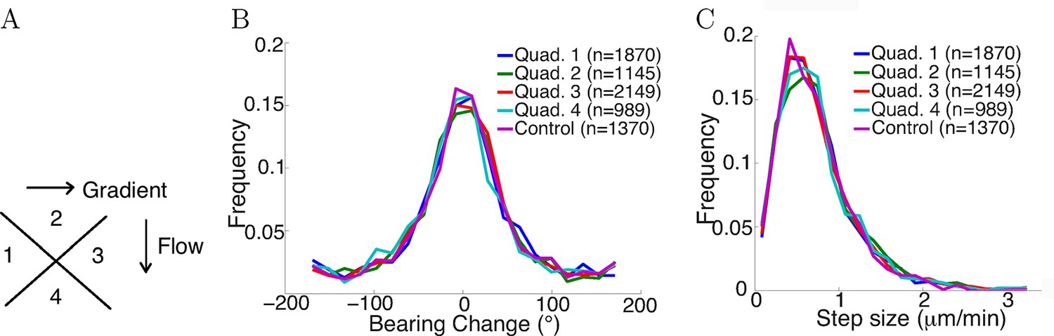
Flow did not affect step statistics.
(A) Axons growing in different directions were grouped into four quadrants. (B) Growth cones’ step sizes in different quadrants. n values refer to the number of steps in each quadrant. There was no significant difference between the quadrants (p = 0.7 Kruskal-Wallis test). (C) Grow cones’ bearing changes in different quadrants (p = 0.4 Kruskal-Wallis test).
-
Figure 6—source data 1
We divided the axons into four quadrants as explained in Figure 6 and measured the bearing changes and stepsizes in each quadrant.
This file contains the step sizes (Sheet 1) and and bearing changes (Sheet 2) in the control condition (Column A) and in each quadrant of the NGF gradient condition (Columns B-E).
- https://doi.org/10.7554/eLife.12248.015
Figure 7
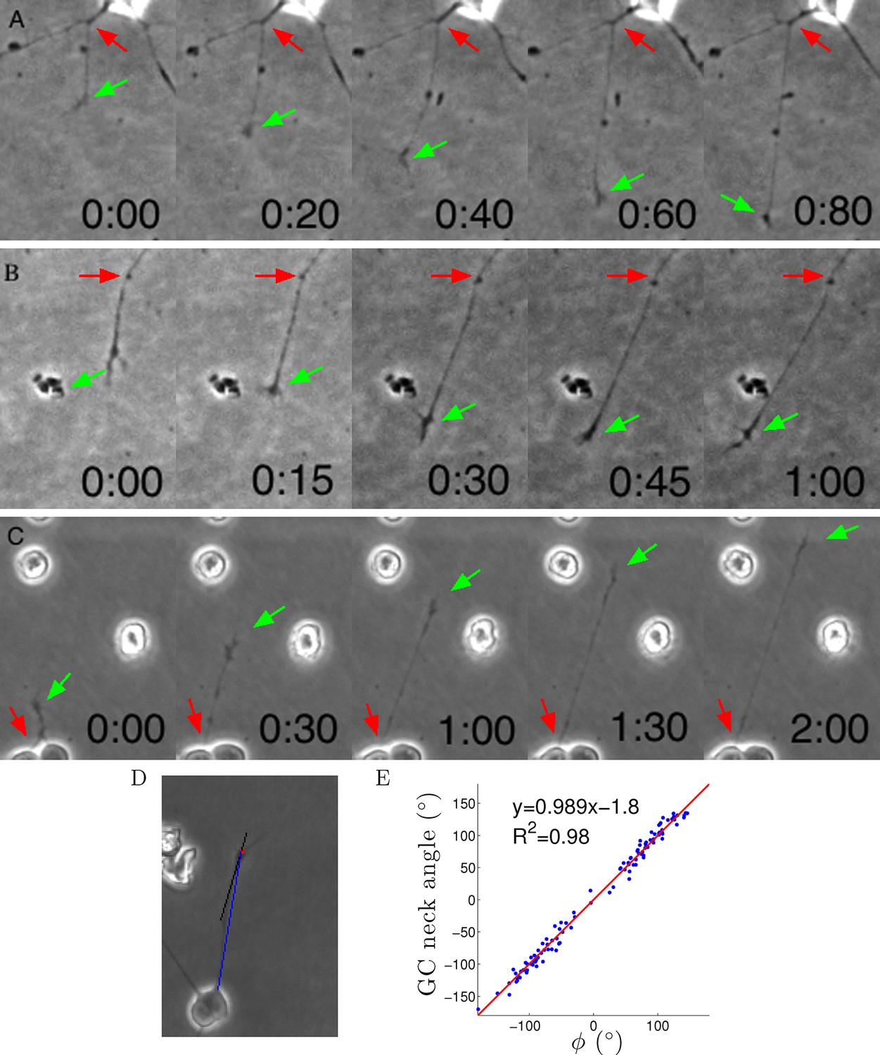
Axons were dragged by growth cones.
(A–C) Timelapse images of three example growth cones. Red arrows point to the putative anchor points and green arrows point to the growth cones. Time is shown in hours and minutes. (D) We measured the angle of the neck of the growth cone (the last 20 μm, black line) and the overall growth cone angle (blue line) after 1 hr from the start of the experiment. (E) The two angles were highly correlated, due to the straightness of the axon.
-
Figure 7—source data 1
We measured the angle of the growth cone from its putative anchor point (Column A) and compared with the angle of the most distal 20 μm segment of the axon (Column B) 1 hr after the start of the experiment.
- https://doi.org/10.7554/eLife.12248.017
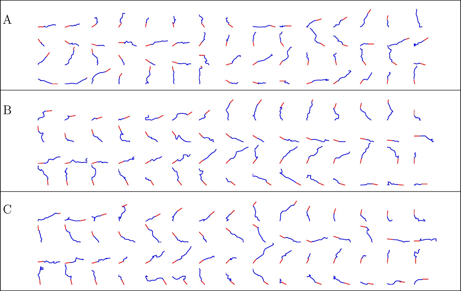
Figure 8

Trajectories of 300 axons growing over 80 min in the control condition, ordered by the initial angle.
The red segments indicate the initial direction of the axon and the blue segments show the traces of the growth cones’ trajectories. Scale bar = 100 μm.
Figure 9
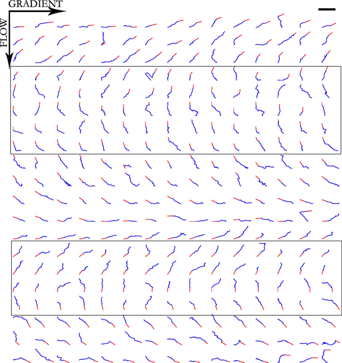
Trajectories of 300 axons growing over 80 min in the NGF gradient, ordered by the initial angle.
Only axons in the box were selected for turning angle measurements as they were almost perpendicular to the gradient, hence most affected by it. Scale bar = 100 μm.
Figure 10
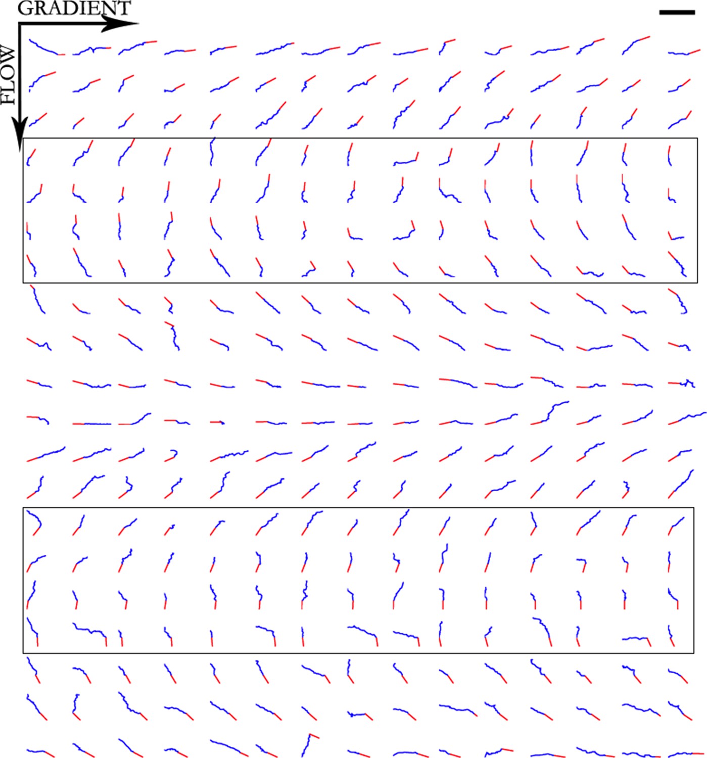
Trajectories of 300 axons growing over 80 min in the NGF gradient with 70 nM KT5720 added, ordered by the initial angle.
Only axons in the box were selected for turning angle measurements. Scale bar = 100 μm.
Figure 11
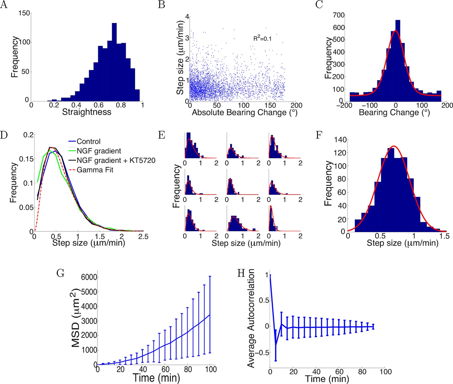
Trajectories were straight with step sizes and bearing changes independent of each other.
(A) Distribution of straightness indices of all paths with mean straightness of 0.72. (B) There was no correlation between bearing change and step size (R2 = 0.1, p = 0.7). (C) The distribution of bearing changes (blue) in radians in the control condition can be fitted to a mixture of two von Mises distributions (red) . (D) Step sizes in the control, attractive and repulsive gradients conditions were similar and well-fitted by the gamma distribution P(x) ∝ x2 exp(−x/24) (red). (E) Step sizes of individual growth cones (blue) can be described by gamma distributions (red) (9 examples shown). (F) This distribution of the average step sizes (blue) of individual growth cones was well-fitted by a Gaussian distribution N(0.7, 0.24) (red). (G) Mean square displacement and standard deviation of 300 growth cones growing over 100 mins in the control condition was super-linear, indicating that growth cone trajectories were straighter than predicted by a simple random walk. (H) Autocorrelation of bearing changes (mean ± std) showed that successive bearing changes were anti-correlated.
-
Figure 11—source data 1
From our 5-min interval tracings, we measured the bearing changes and step sizes in the control condition (Columns A, B), the mean step sizes of all the growth cones (Column C) and the step sizes in the NGF gradient and NGF gradient + KT5720 conditions (Columns D,E).
- https://doi.org/10.7554/eLife.12248.025
Figure 12
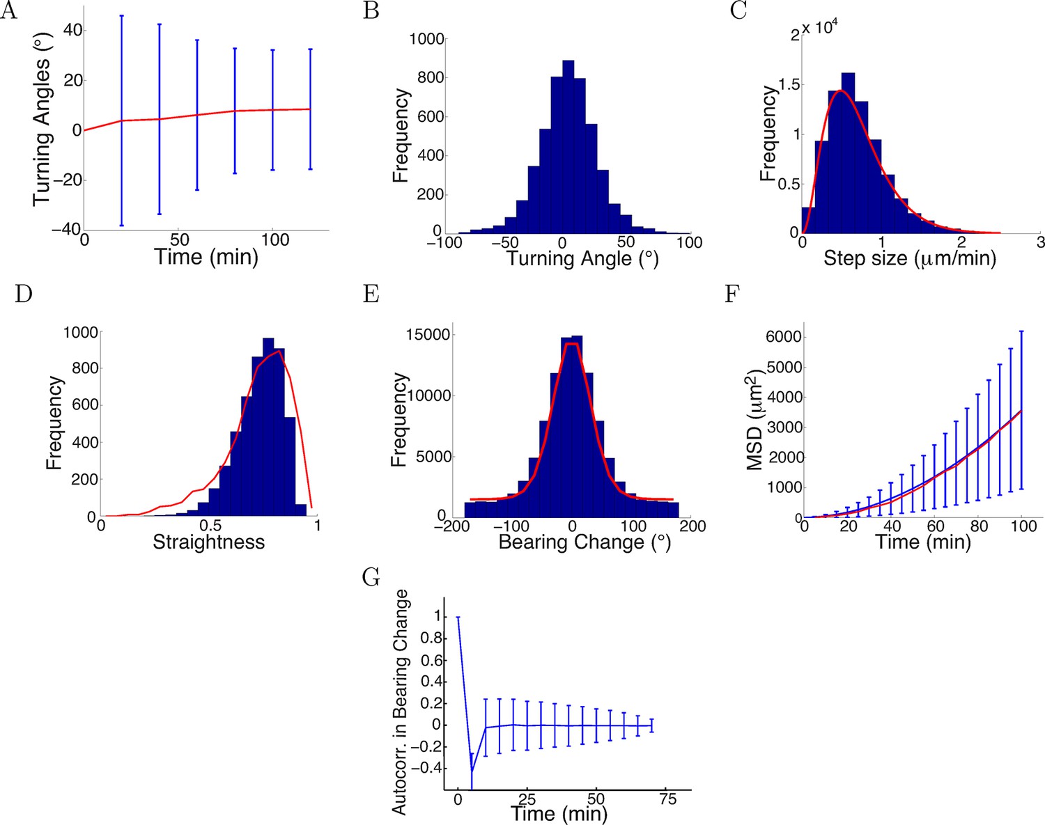
Model captured key statistics of trajectories.
(A) The evolution of simulated turning angles (mean ± std) of n=5000 growth cones over time in the attractive gradient condition. (B) Simulated turning angles after 16 steps (80 min) had mean 9.8° and standard deviation of 24.2°, similar to the empirical data in red in Figure 4B. (C) Distribution of simulated step lengths (blue), fitted with the empirical distribution (red). (D) Straightness of simulated trajectories (mean 0.75, blue), compared with empirical distribution (red) (p = 0.2, t-test). (E) Simulated bearing changes (blue) fitted with the mixture of von Mises distributions given in Figure 11D (red). (F) Mean square displacement of simulations (blue) and data (red). (G) Autocorrelation of simulated bearing changes.
-
Figure 12—source code 1
The code to simulate the trajectories based on Equation 1 with the step sizes and bearing changes described in Section Turning angles over time were well predicted by the model.
- https://doi.org/10.7554/eLife.12248.027
Figure 13
Simulated trajectories from three conditions.
(A) control, (B) NGF gradient, (C) NGF gradient + KT5720.
Figure 14
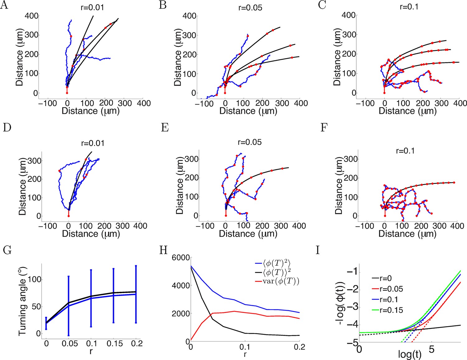
More variability with more anchor points.
(A–C) Trajectories of growth cones with probability of putting down a new anchor r= 0.01, 0.05, 0.1 at each timestep and the same parameters as Figure 2A (a = 1, b = 0.1, T = 150 timesteps). The black plots are without noise in the bearing changes, the blue plots are with noise radians in the bearing changes and the red dots are the anchor points. More anchor points lead to higher variability but also stronger turning. The means and standard deviations of turning angles and the values for the noiseless versus the noisy case in brackets for r = 0.01, 0.05, 0.1 are 32 ± 9° (30 ± 36°), 55 ± 8° (49 ± 57°) and 67 ± 5° (60 ± 56°), respectively. (D–F) Trajectories of growth cones with the same rate of putting down new anchor points as A-C but at regular intervals. The means and standard deviations of turning angles and the values for the noiseless versus the noisy case in brackets are 27° (24 ± 17°), 57° (54 ± 51°), 69° (66 ± 51°). (G) The means and standard deviations of turning angles after 150 timesteps as a function of the anchoring rate at regular intervals in the noiseless and the noisy case. (H) The mean square of the final growth cone angle (in degrees) for different anchoring rates r after 150 steps. is the sum of the bias term and the variance term var(). Although more anchor points add more variance to the final angle (red curve), they achieve stronger turning (black curve). (I) The evolution of over time, for the case of anchoring at regular intervals and no noise in the movement (ξ = 0). With more anchor points, also follows the power law but with steeper slope, meaning that at a faster rate than the case without anchor points.
-
Figure 14—source code 1
The code to simulate the trajectories based on Equation 1 with normally distributed noise in bearing changes described in Section Multiple anchor points achieved sharp turns but also increased variability.
In the regular anchoring case, the growth cone position after every 1/r steps becomes a new anchor point. In the probabilistic anchoring case, each growth cone position has a probability of r to become a new anchor point.
growth-cone-tracker-5min. Growth cone tracking code. The code tracks the position of the growth cone centre every 5 mins from timelapse AVI files.
extract-GC-positions. Growth cone position extraction code. The code to extract the position of the growth cone from the tracings.
- https://doi.org/10.7554/eLife.12248.030
Videos
Video 1
Timelapse images of an example growth cone.
One-minute interval phase contrast timelapse imaging of a growth cone in a microfluidic chamber.
Video 2
Timelapse images of an example growth cone.
One-minute interval phase contrast timelapse imaging of a growth cone in a microfluidic chamber.
Video 3
Timelapse images of an example growth cone.
One-minute interval phase contrast timelapse imaging of a growth cone in a microfluidic chamber.
Tables
Table 1
Summary of model parameters (GC: growth cone).
| Symbol | Meaning |
| GC’s current bearing | |
| GC’s overall angle | |
| Gradient direction | |
| Bearing change | |
| Turning angle after 80 min | |
| Persistence strength | |
| Bias strength | |
| Noise in bearing change | |
| Standard deviation of | |
| Step size every 5 min | |
| Distance from origin to GC | |
| Straightness index | |
| Anchoring rate |
Download links
A two-part list of links to download the article, or parts of the article, in various formats.
Downloads (link to download the article as PDF)
Open citations (links to open the citations from this article in various online reference manager services)
Cite this article (links to download the citations from this article in formats compatible with various reference manager tools)
RETRACTED: A mathematical model explains saturating axon guidance responses to molecular gradients
eLife 5:e12248.
https://doi.org/10.7554/eLife.12248


