A simple generative model of the mouse mesoscale connectome
- National Institutes of Health, United States
- Newcastle University, United Kingdom
- University of Washington, United States
Figures
Figure 1
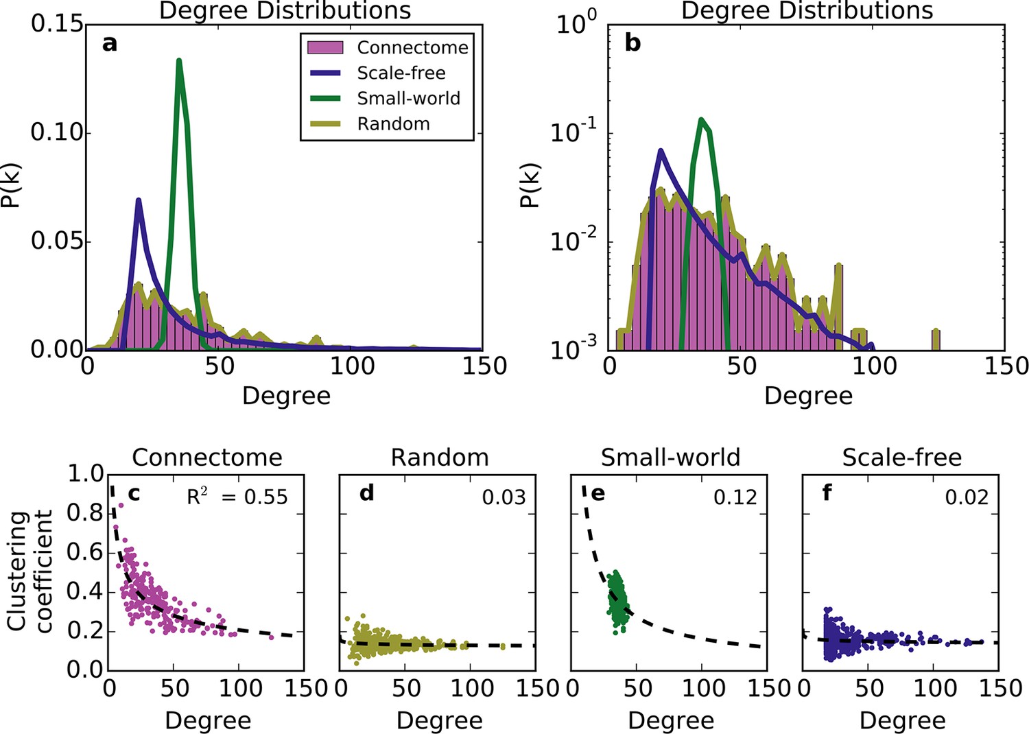
Standard graph models vary in their ability to recreate the mouse connectome’s degree distribution and relationship between degree and clustering coefficient.
(a-b) Probability density of degree distributions for the mouse connectome, and an average over 100 repeats of scale-free, small-world, and (degree-controlled) random networks plotted with (a) linear and (b) log-linear scales. (c-f) Clustering coefficient as a function of degree for each node in (c) the mouse connectome, (d) a degree-controlled random network, (e) a small-world network, and (f) a scale-free network. Each plot shows data from 426 nodes and the best fitting power law function (dashed line). (a) is similar to Figure 3c from Oh et al. (2014).
Figure 2
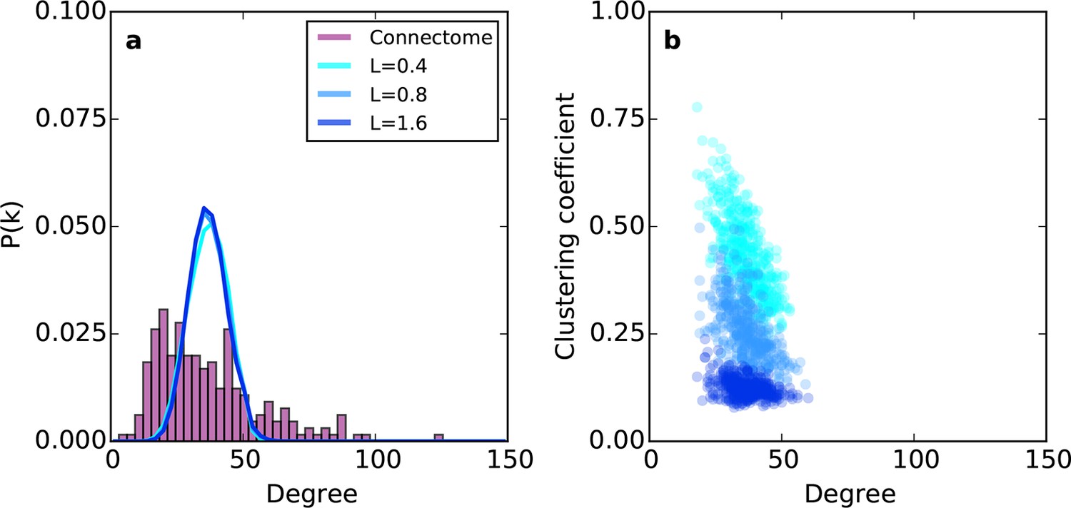
Example networks generated using the (purely geometric) proximal attachment (PA) rule where connection probability between two nodes decreased with distance.
(a) The degree distribution for networks grown with three values of L (in mm), each averaged across 100 repeats. The mouse connectome is shown for comparison. (b) Clustering coefficient as a function of degree for representative networks grown with the same values of L used in (a).
Figure 3 with 1 supplement
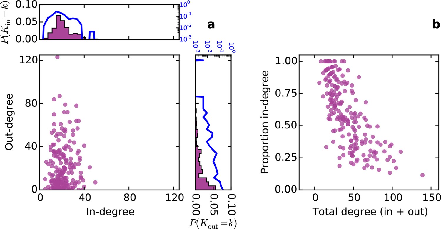
Directed analysis of the mouse connectome reveals different distributions for in- and out-degree.
(a) Out-degree as a function of in-degree for all nodes in the mouse connectome. Margins show in- and out-degree distributions with the blue lines and axis labels corresponding to a logarithmic scale. In-degree is approximately normally distributed while the out-degree approximately follows an exponential distribution. (b) Proportion in-degree as a function of total degree (i.e. in-degree divided by the sum of incoming and outgoing edges). Low-degree nodes tend to have mostly incoming edges, whereas high-degree nodes are characterized by mostly outgoing edges.
Figure 3—figure supplement 1

Distribution of proportion in-degree in the mouse connectome.
https://doi.org/10.7554/eLife.12366.006
Figure 4
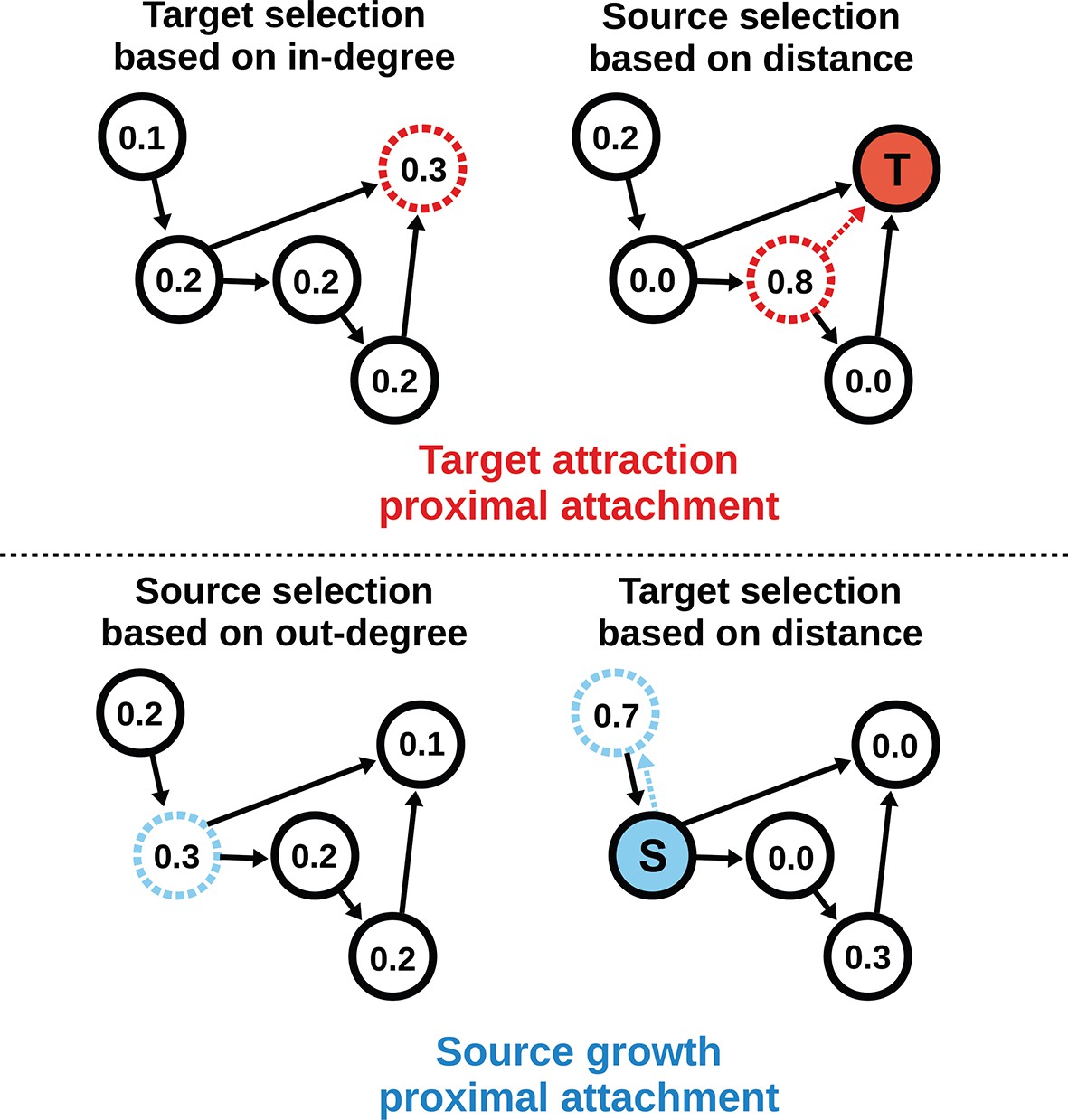
Target attraction and source growth network generation algorithms.
The numbers inside each node indicate the probability of growth or attachment. For illustration, the most probable node (dashed) is selected in both diagrams (T and S, corresponding to target and source, respectively). Top row: target attraction proximal attachment (TAPA) model. A target node is selected with a probability proportional to its in-degree (left), while the source node is chosen with a probability that decreases exponentially with the node’s Euclidean distance from the target (right). Two nodes have zero probability of forming an edge since the target is already receiving projections from these nodes. The dashed red line shows the most probable edge. Bottom row: source growth proximal attachment (SGPA) model. A source node is selected with a probability proportional to its out-degree (left), while the target node is chosen with a probability that decreases exponentially with the node’s Euclidean distance from the source (right). The dashed cyan line shows the most probable edge. In both algorithms, we assume that each node begins with a self-connection (corresponding to an outgoing and incoming edge) to avoid zero-valued probabilities, though self-connections are not shown here or included when calculating any metrics.
Figure 5 with 5 supplements
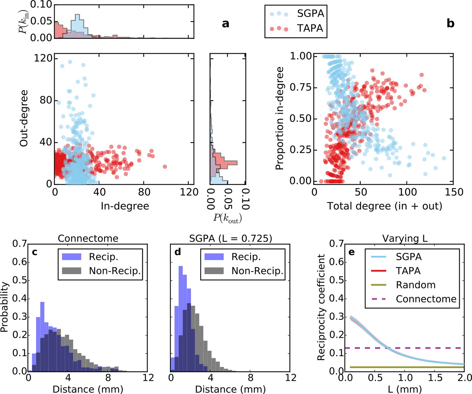
Directed analysis of single representative TAPA and SGPA network models and reciprocity comparison with the connectome.
(a) Out-degree as a function of in-degree for both algorithms with L = 0.725 mm, which was chosen to match the connectome’s reciprocity ‒ see e). Margins show in- and out-degree distributions. (b) Proportion in-degree as a function of total degree for both algorithms. The SGPA model qualitatively captures the connectome’s directed degree distributions and proportion in-degree (cf. Figure 2). (c) Edge length distribution for the connectome, shown for both reciprocal (blue) and non-reciprocal edges (black). (d) Same as (c) but for the SGPA model. (e) Reciprocity coefficient as a function of the length parameter for both TAPA (red) and SGPA (cyan), with shading indicating standard deviation over 100 repeats. Both models intersect the connectome at L = 0.725 mm. For reference, the reciprocity coefficient for the connectome (magenta) and a corresponding degree-controlled random graph (gold) are also shown. SGPA and TAPA models overlap.
Figure 5—figure supplement 1
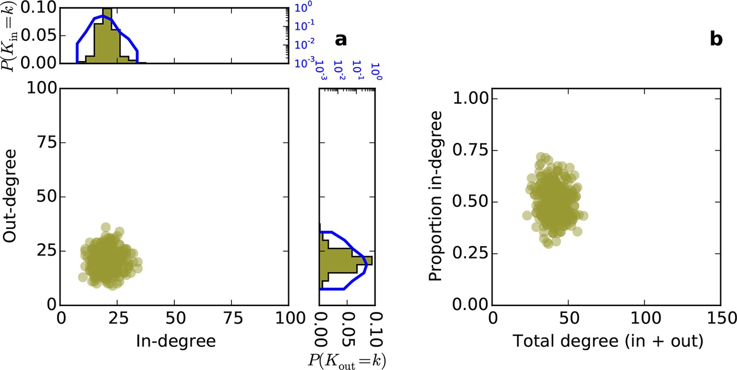
Directed degree distributions and proportion in-degree for a directed Erdos-Renyi graph.
(a) In- and out-degree are independent and both are approximately normally distributed. (b) Proportion in-degree is independent of total degree.
Figure 5—figure supplement 2
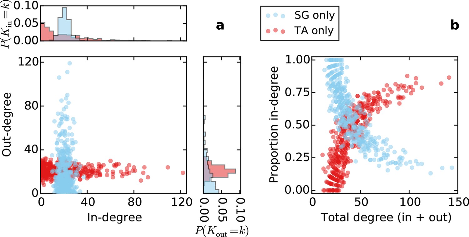
Directed degree distributions and proportion in-degree for a purely topological source-growth or target-attraction directed graph (SG only, TA only, respectively), with no proximal attachment (equivalent to L = ∞ in SGPA or TAPA).
The qualitative properties of the in- and out-degree distributions are the same as in SGPA and TAPA with L = 0.725.
Figure 5—figure supplement 3
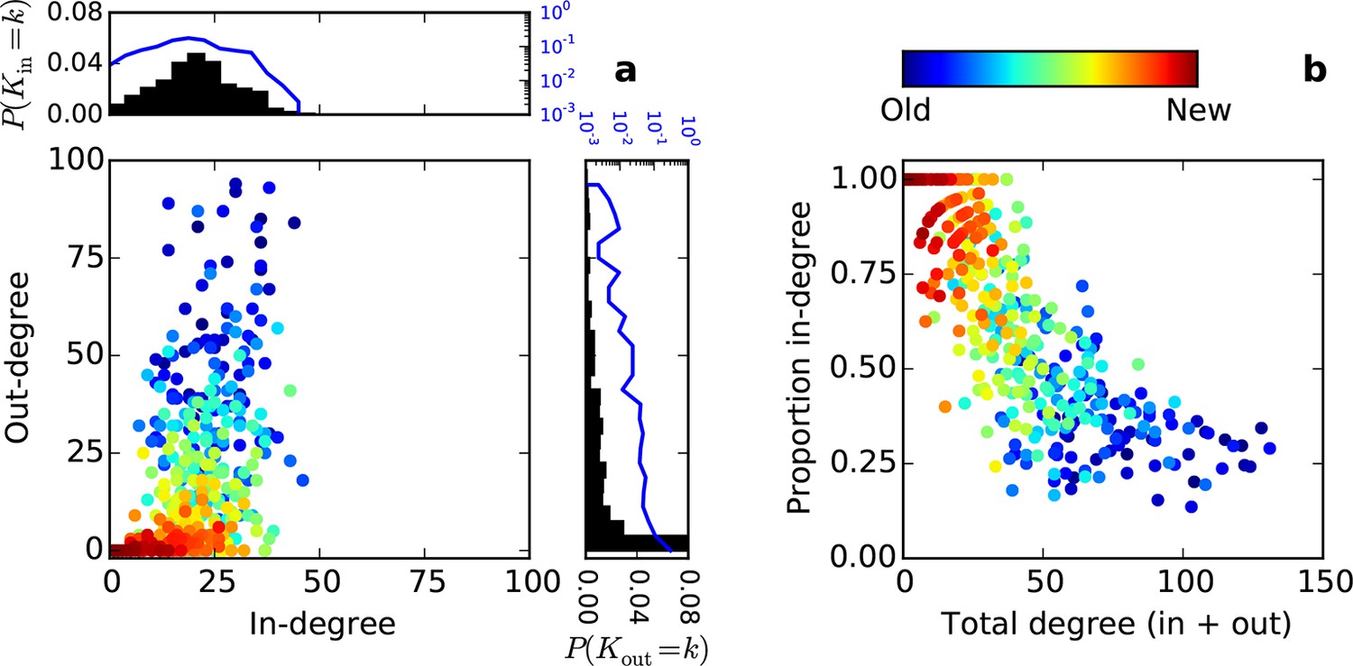
Directed degree distributions and proportion in-degree for an SGPA model where the network is grown one node at a time.
Hotter colors indicate more recently added nodes. (a) Out- and in-degree relationships for one representative model instantiation with L = 0.725 mm. (b) Proportion in-degree as a function of total degree.
Figure 5—figure supplement 4
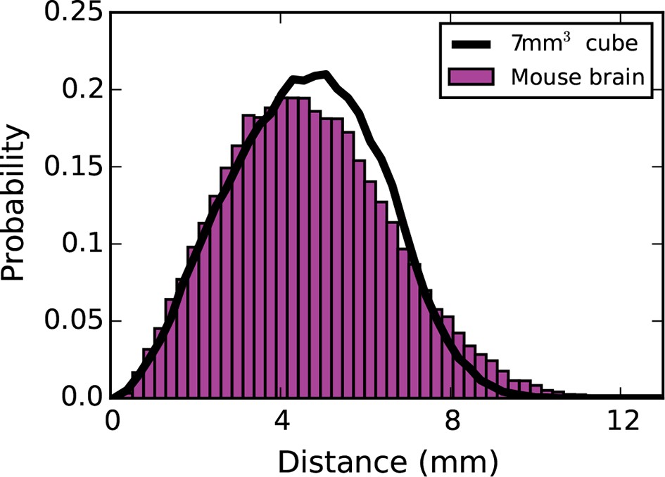
Inter-nodal distance distribution for the mouse brain (magenta bars) and a 7 mm³ cube (black line).
The use of a 7 mm x 7 mm x 7 mm cube was justified on the basis that its inter-nodal distance distribution closely mimicked that of the connectome. The results did not change considerably when coordinates from the mouse brain were used instead of the 7 mm³ cube.
Figure 5—figure supplement 5

Directed degree distributions and proportion in-degree for a graph in which source selection was proportional to total degree (in-degree + out-degree) in (a) and (b), and in which source selection was proportional to total degree raised to the power γ = 1.67 in (c) and (d).
In both (a) and (c), there are significant correlations between the in- and out-degrees (ρ = 0.45, p< 10-10 and ρ = 0.60, p < 10-10 for (a) and (b), respectively; Spearman rank correlation). In all graphs, L = 0.725 mm.
Figure 6 with 3 supplements
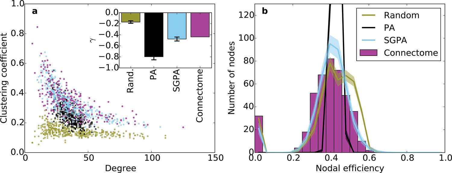
Clustering and nodal efficiency for the connectome and other directed models.
(a) Clustering-degree joint distribution for connectome and one representative instantiation of each model graph. Inset: best-fit power-law exponent (see 'Materials and methods') for the connectome ( = -0.44, ) and random (mean ± std. = -0.17 ± 0.02, median ), SGPA (mean ± std. = -0.48 ± 0.04, median ), and geometric PA (mean ± std. = -0.80 ± 0.06, median ) models. (b) Distributions of nodal efficiencies (see 'Materials and methods') with mean ± standard deviation (line and shaded regions, respectively) for model networks. Mean ± standard deviation of mean nodal efficiency (averaged over nodes) is 0.409 ± 0.001 for the random model, 0.393 ± 0.004 for the SGPA model, and 0.426 ±. 001 for the pure geometric model. The connectome’s average nodal efficiency is 0.375. The PA model’s histogram peaks at 279 at a nodal efficiency of 0.44. (b) and the inset in a) both used 100 sample instantiations of each model.
Figure 6—figure supplement 1

Clustering and nodal efficiency for Erdos-Renyi (ER) and TAPA models.
(a) Clustering-degree joint distribution for connectome and one representative instantiation of each model graph. The inset shows best-fit power-law exponents, as in Figure 6 (ER: mean ± std. = -0.01 ± 0.04, median R2 = 0.00; TAPA: mean ± std. = -0.47 ± 0.035, median R2 = 0.60). (b) Distributions of nodal efficiencies (see 'Materials and methods'). Solid lines are means and shaded regions are standard deviations. (b) and the inset in (a) both used 100 sample instantiations of each model. Mean ± standard deviation (taken over 100 graph instantiations) of mean nodal efficiency (averaged over nodes) is 0.467 ± 0.002 for ER, 0.395 ± 0.003 for TAPA.
Figure 6—figure supplement 2
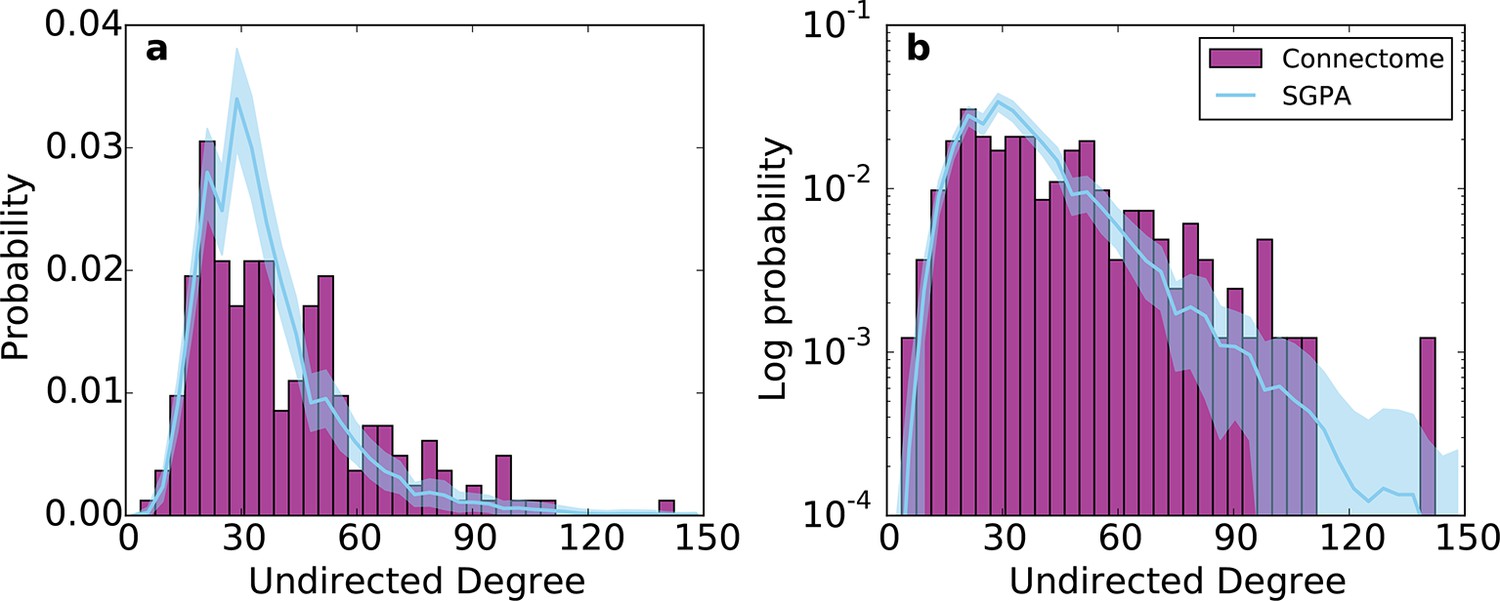
Undirected degree distribution for the SGPA model and the mouse connectome in (a) linear and (b) logarithmic scales.
For the SGPA model, the line and shaded region represent the mean and standard deviation across 100 graph instantiations.
Figure 6—figure supplement 3
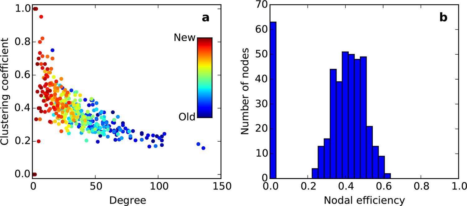
Clustering vs. degree (a) and nodal efficiency (b) for the node-by-node SGPA network (L = 0.725) used in Figure 5—figure supplement 3.
Hotter colors indicate more recently added nodes.
Figure 7 with 1 supplement
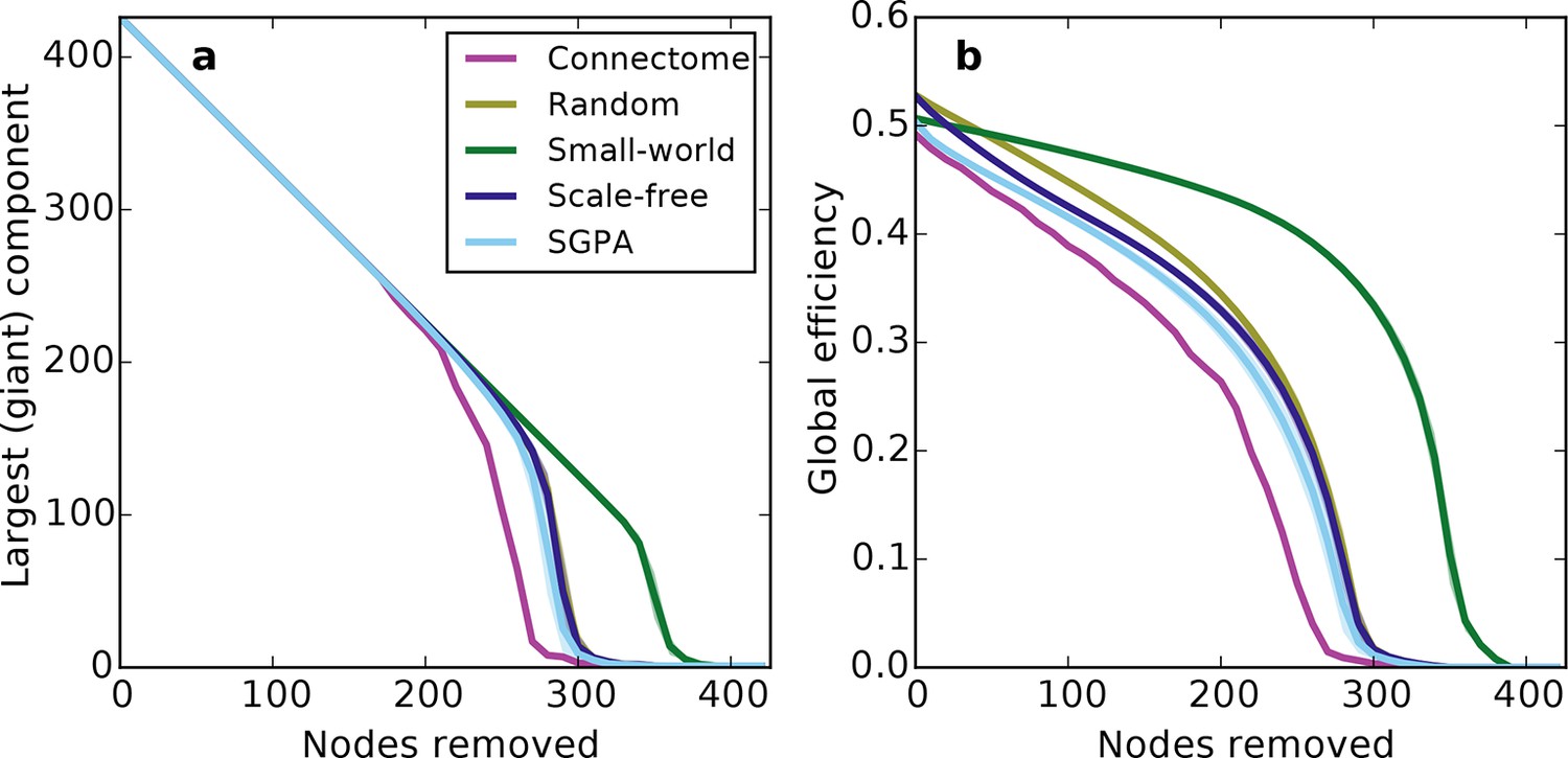
Response of undirected networks to targeted lesions where nodes are removed in order of highest degree.
Mean values (lines) ± standard deviations (shaded regions) are plotted for each model after 100 repeats. (a) Size of the largest (giant) connected component in response to targeted attack. The randomly shuffled connectome (Random) is obscured by the scale-free graph. (b) Global efficiency for the mouse connectome and network models in response to targeted attack.
Figure 7—figure supplement 1
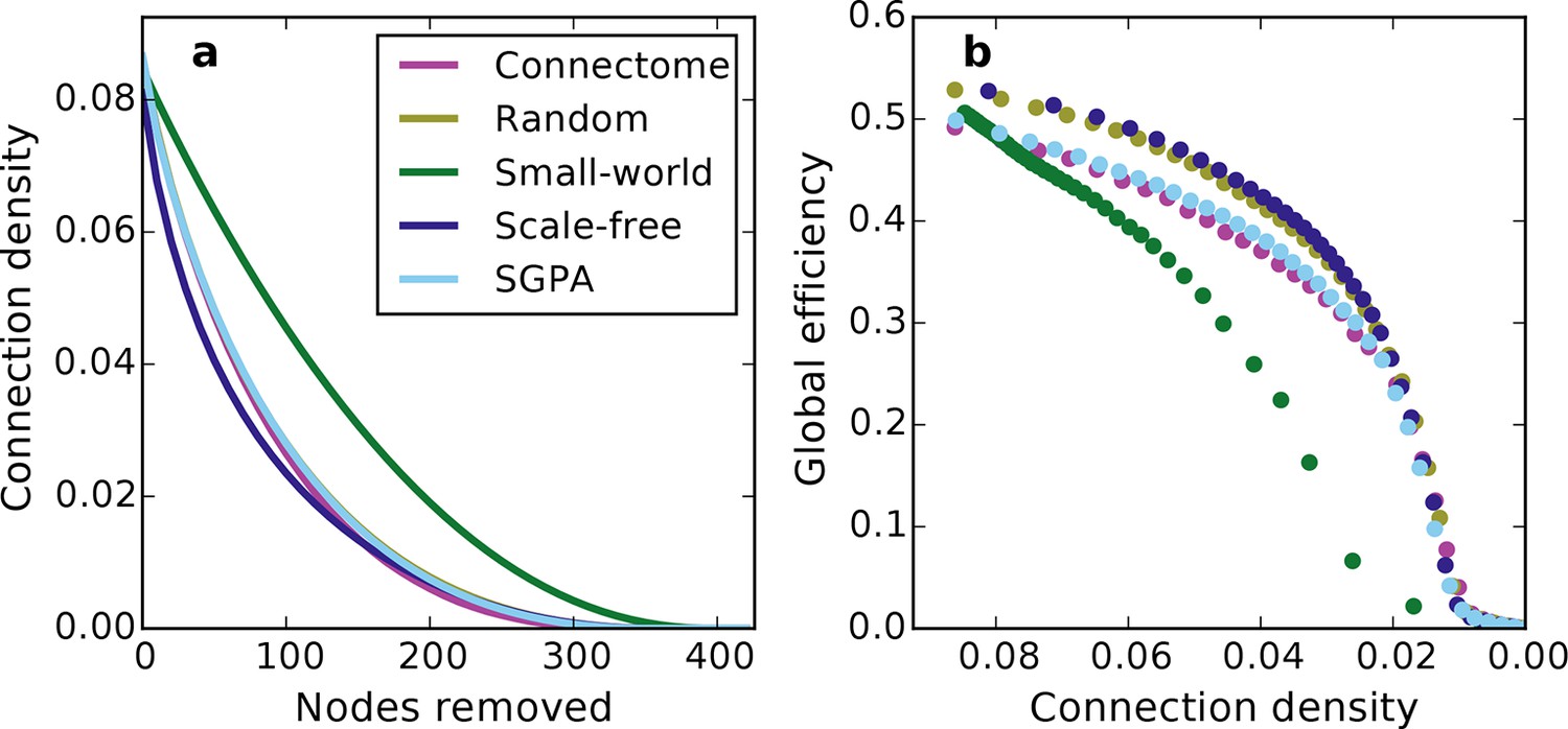
Network connectivity patterns (and not just connection density) affect global efficiency.
(a) Connection density as a function of nodes removed (for comparison with Figure 7). Except for the small-world network, the connection density was changed similarly throughout the lesioning process. Mean values (lines) ± standard deviations (shaded regions) are plotted for each model after 100 repeats. (b) Global efficiency and connection density at each point during the lesioning process for representative networks grown in the same manner as Figure 7. Note that global efficiency varies across graphs even at similar connection densities.
Tables
Table 1
Average undirected metrics for the connectome, standard, and model networks. For the random, small-world, scale-free, and SGPA models, the standard deviation for 100 repeats is also shown. See Table 2 for metric definitions. Note that properties for the original (single-hemisphere) connectome are presented in Oh et al. (2014).
| Clustering | Characteristic path length | Global efficiency | |
|---|---|---|---|
| Connectome | 0.361 | 2.226 | 0.492 |
| Random | 0.140 ± 0.0013 | 2.002 ± 0.0020 | 0.528 ± 0.0003 |
| Small-world | 0.359 ± 0.0058 | 2.129 ± 0.0058 | 0.507 ± 0.0010 |
| Scale-free | 0.159 ± 0.0037 | 1.998 ± 0.0026 | 0.527 ± 0.0004 |
| SGPA | 0.343 ± 0.0094 | 2.166 ± 0.0159 | 0.501 ± 0.0027 |
Table 2
Graph theoretical metrics used for analysis.
| Metric | Brief interpretation | Definition |
|---|---|---|
| Degree | Number of edges connected to a node. This generalizes to in- or out-degree in directed graphs, describing the number of incoming or outgoing connections for a node, respectively. | Directed versions: |
| Clustering coefficient (Watts and Strogatz, 1998) | Level of connectivity among nearest neighbors of node | |
| Characteristic path length (Watts and Strogatz, 1998) | Mean shortest undirected path length over all pairs of nodes | |
| Global efficiency (Latora and Marchiori, 2001) | Mean inverse shortest undirected path length over all pairs of nodes | |
| Nodal efficiency (generalized from [Achard and Bullmore, 2007]) | Mean inverse shortest directed path length from a single node to all other nodes | |
| Reciprocity coefficient | Proportion of edges from node to node that have a reciprocal connection from node to node (when ) | |
Download links
A two-part list of links to download the article, or parts of the article, in various formats.
Downloads (link to download the article as PDF)
Open citations (links to open the citations from this article in various online reference manager services)
Cite this article (links to download the citations from this article in formats compatible with various reference manager tools)
A simple generative model of the mouse mesoscale connectome
eLife 5:e12366.
https://doi.org/10.7554/eLife.12366


