Figures and data in Optimal compensation for neuron loss | eLife

Figures

9 figures

Figures

Figure 1

Download asset Open asset

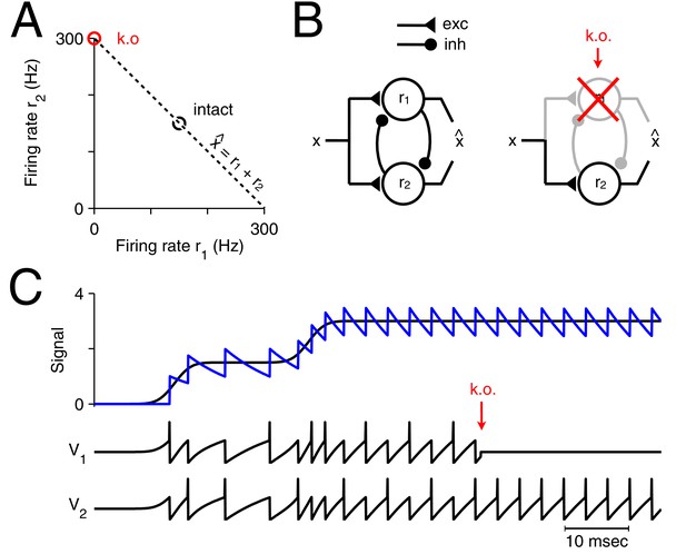
Optimal representation and optimal compensation in a two-neuron example.

(A) A signal $x$ can be represented using many different firing rate combinations (dashed line). Before cell loss, the combination that best shares the load between the neurons, requires that both cells are equally active (black circle). After the loss of neuron 1, the signal must be represented entirely by the remaining neuron, and so, its firing rate must double (red circle). We will refer to this change in firing rate as an optimal compensation for the lost neuron. (B) This optimal compensation can be implemented in a network of neurons that are coupled by mutual inhibition and driven by an excitatory input signal. When neuron 1 is knocked out, the inhibition disappears, allowing the firing rate of neuron 2 to increase. (C) Two spiking neurons, connected together as in B, represent a signal $x$ (black line, top panel) by producing appropriate spike trains and voltage traces, $V_{1}$ and $V_{2}$ (lower panels). To read out the original signal, the spikes are replaced by decaying exponentials (a simple model of postsynaptic potentials), and summed to produce a readout, $\hat{x}$ (blue, top panel). After the loss of neuron 1 (red arrow), neuron 2 compensates by firing twice as many spikes.

https://doi.org/10.7554/eLife.12454.002

Figure 2

Download asset Open asset

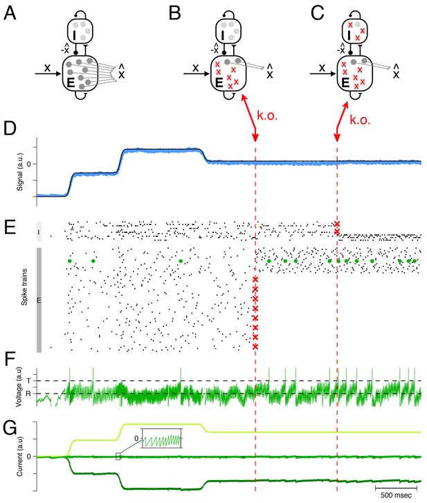
Optimal compensation in a larger spiking network with separate excitatory (E) and inhibitory (I) populations ( $N = 80$ excitatory and $N = 20$ inhibitory neurons) (A) Schematic of network representing a scalar signal $x (t)$ .

The excitatory neurons receive an excitatory feedforward input, that reflects the input signal, $x (t)$ , and a recurrent inhibitory input, that reflects the signal estimate, $\hat{x} (t)$ . The signal estimate stems from the excitatory population and is simply re-routed through the inhibitory population. In turn, the voltages of the excitatory neurons are given by a transformation of the signal representation error, $V_{i} = D_{i} (x (t) - \hat{x} (t))$ , assuming that $β = 0$ . Since a neuron’s voltage is bounded from above by the threshold, all excesses in signal representation errors are eliminated by spiking, and the signal estimate remains close to the signal, especially if the input signals are large compared to the threshold. Mechanistically, excitatory inputs here generate signal representation errors, and inhibitory inputs eliminate them. The prompt resolution of all errors is therefore identical to a precise balance of excitation and inhibition. (B) Schematic of a network with 75% of the excitatory neurons knocked out. (C) Schematic of a network with 75% of the inhibitory neurons knocked out also. (D) The network provides an accurate representation $\hat{x} (t)$ (blue line) of the time-varying signal $x (t)$ (black line). Whether part of the excitatory population is knocked out or part of the inhibitory population is knocked out, the representation remains intact, even though the readout weights do not change. (E) A raster plot of the spiking activity in the inhibitory and excitatory populations. In both populations, spike trains are quite irregular. Red crosses mark the portion of neurons that are knocked out. Whenever neurons are knocked out, the remaining neurons change their firing rates instantaneously and restore the signal representation. (F) Voltage of an example neuron (marked with green dots in E) with threshold $T$ and reset potential $R$ . (G) The total excitatory (light green) and inhibitory (dark green) input currents to this example neuron are balanced, and the remaining fluctuations (inset) produce the membrane potential shown in F. This balance is maintained after the partial knock-outs in the E and I populations.

https://doi.org/10.7554/eLife.12454.003

Figure 3

Download asset Open asset

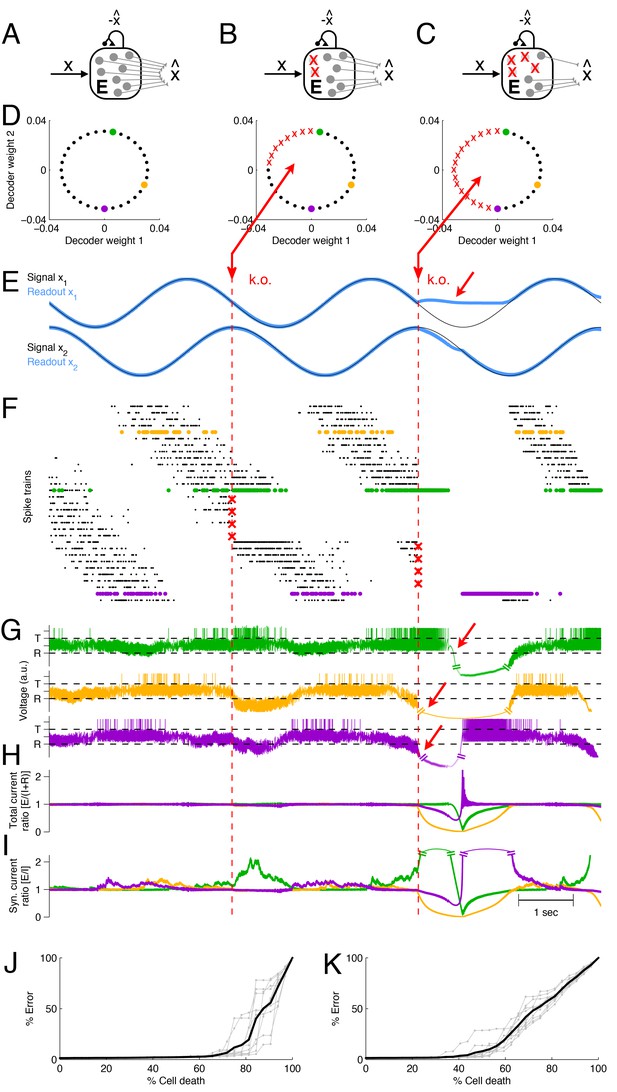
Optimal compensation and recovery boundary in a network with $N = 32$ excitatory neurons representing a two-dimensional signal $𝐱 (t) = (x_{1} (t), x_{2} (t))$ .

(A–C) Schematic of network and knock-out schedule. (Inhibitory neurons not explicitly modeled for simplicity, see text.) (B) Neural knock-out that leads to optimal compensation. (C) Neural knock-out that pushes the system beyond the recovery boundary. (D) Readout or decoding weights of the neurons. Since the signal is two-dimensional, each neuron contributes to the readout with two decoding weights, shown here as black dots. Red crosses in the central and right panel indicate neurons that are knocked out at the respective time. (E) Signals and readouts. In this example, the two signals (black lines) consist of a sine and cosine. The network provides an accurate representation (blue lines) of the signals, even after 25% of the neurons have been knocked out (first dashed red line). When 50% of the neurons are knocked out (second dashed red line), the representation of the first signal fails temporarily (red arrow). (F) A raster plot of the spiking activity of all neurons. Neurons take turns in participating in the representation of the two signals (which trace out a circle in two dimensions), and individual spike trains are quite irregular. Red crosses mark the portion of neurons that are knocked out. Colored neurons (green, yellow, and purple dots) correspond to the neurons with the decoder weights shown in panel D. Note that the green and purple neurons undergo dramatic changes in firing rate after the first and second knock-outs, respectively, which reflects their attempts to restore the signal representation. (G) Voltages of the three example neurons (marked with green, yellow, and purple dots in D and F), with threshold $T$ and reset potential $R$ . (H) Ratio of positive (E; excitation) and negative (I+R; inhibition and reset) currents in the three example neurons. After the first knock-out, the ratio remains around one, and the system remains balanced despite the loss of neurons. After the second knock-out, part of the signal can no longer be represented, and balance in the example neurons is (temporarily) lost. (I) Ratio of excitatory and inhibitory currents. Similar to H, except that a neuron’s self-reset current is not included. (J) When neurons are knocked out at random, the network can withstand much larger percentages of cell loss. Individual grey traces show ten different, random knock-out schemes, and the black trace shows the average. (K) When neurons saturate, the overall ability of the network to compensate for neuron loss decreases.

https://doi.org/10.7554/eLife.12454.004

Figure 4 with 3 supplements

Download asset Open asset

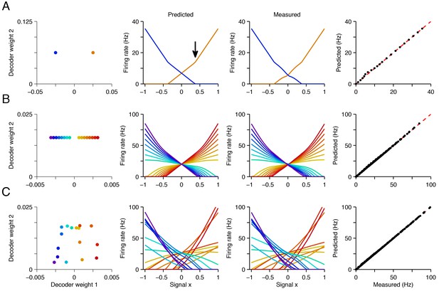
Explaining tuning curves in the spiking network with quadratic programming.

(A) A network with $N = 2$ neurons. The first column shows the decoding weights for the two neurons. The first decoding weight determines the readout of the signal $x_{1} = x$ , whereas the second decoding weight helps to represent a constant background signal $x_{2} = r_{B}$ . The second column shows the tuning curves, i.e., firing rates as a function of $x$ , predicted using quadratic programming. The third column shows the tuning curves measured during a 1 s simulation of the respective spiking network. The fourth column shows the match between the measured and predicted tuning curves. (B) Similar to A , but using a network of $N = 16$ neurons with inhomogeneous, regularly spaced decoding weights. The resulting tuning curves are regularly spaced. Neurons with small decoding weight magnitude have eccentric firing rate thresholds and shallow slopes; neurons with large decoding weight magnitudes have central firing rate thresholds and steep slopes. (C) Similar to B except that decoding weights and cost terms are irregularly spaced. This irregularity leads to inhomogeneity in the balanced network tuning curves, and in the quadratic programming prediction (see also Figure 4—figure supplements 1–3).

https://doi.org/10.7554/eLife.12454.005

Figure 4—figure supplement 1

Download asset Open asset

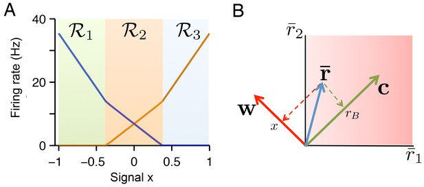
The geometry of quadratic programming.

(A) Tuning curves calculated for a two neuron example. The tuning curve solution can be decomposed into three regions: region $ℛ_{1}$ where ${\bar{r}}_{1} = 0$ and ${\bar{r}}_{2} \geq 0$ , region $ℛ_{2}$ where ${\bar{r}}_{1} \geq 0$ and ${\bar{r}}_{2} \geq 0$ , and region $ℛ_{3}$ where ${\bar{r}}_{2} = 0$ and ${\bar{r}}_{1} \geq 0$ . In each region the firing rate solution is given by a different linear projection of $𝐱^{'} = (x, r_{B})$ , where $r_{B}$ is a fixed background signal. (B) If the readout vectors of the two neurons are defined as $D_{1} = (w, c)$ and $D_{2} = (- w, c)$ , then the transformation from firing rate space to signal space is given by a simple linear projection of firing rates onto the vectors $w = (- w, w)$ (for the variable signal $x$ ) and $c = (c, c)$ (for the background signal). Unlike the transformation from signal space to firing rate space in A , this transformation is not region dependent.

https://doi.org/10.7554/eLife.12454.006

Figure 4—figure supplement 2

Download asset Open asset

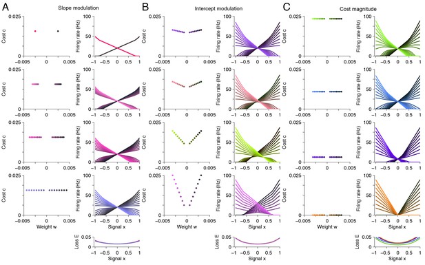
A taxonomy of tuning curve shapes.

Here, we explore the relationship between tuning curve shape and the choice of readout weights for the variable signal (‘weight’ $w$ ) and the background signal (‘cost’ $c$ ). Specifically, we calculate tuning curve shape using quadratic programming for 12 distinct systems, each with different parameter values. (A) The left column shows the read-out weights $D_{i} = (w_{i}, c_{i})$ for each system. The right column shows the tuning curves calculated using quadratic programming. Each row corresponds to a distinct neural population. In this panel, we increase the spread of the read-out weight $w_{i}$ from top to bottom (left column), and we find that the range of tuning curve slopes increase (right column). The loss is approximately invariant to this modulation (right column, bottom). (B) Similar to A , except that we increase the spread of the read-out weights $c_{i}$ (‘cost’ term) from top to bottom (left column), and we observe that the range of tuning curve intercept values increase (right column). Again, the loss is approximately invariant to this modulation (right column, bottom). (C) Similar to A and B except that this time we reduce the magnitude of the read-out weights $c_{i}$ from top to bottom (left column), and we observe that the intercept values decrease, until tuning curves do not overlap with each other (right column). This time, the loss increases marginally (right column, bottom). This happens because the system is unable to represent the background signal.

https://doi.org/10.7554/eLife.12454.007

Figure 4—figure supplement 3

Download asset Open asset

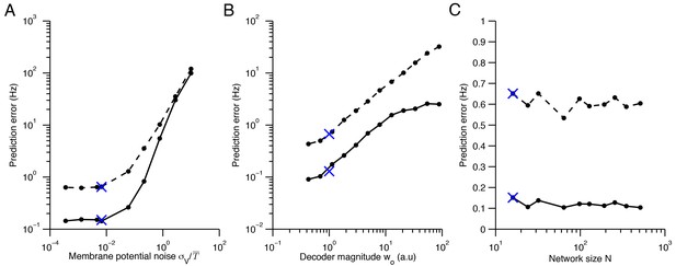
Quadratic programming firing rate predictions compared to spiking network measurements.

(A) The impact of membrane potential noise $σ_{V}$ on firing rate predictions is calculated by comparing quadratic programming predictions and firing rate measurements in network simulations. We calculate the prediction error of quadratic programming by taking the average absolute difference between quadratic programming predictions and spiking network measurements (solid line) and by taking the standard deviation of these measurements about the predictions (dashed line). Averages are calculated across neurons, stimuli and time, using networks with tuning curve shapes similar to Figure 5B. In the parameter range used throughout this paper (indicated by a blue cross), the prediction error is small and robust to changes in noise. As expected, the error increases when the noise is the same order of magnitude as the mean spiking threshold, $\bar{T} \equiv \sum_{i} T_{i} / N$ . (B) Similarly, the prediction error increases as the size of the decoder weights increase. Here, $α$ is a scaling parameter that characterizes the magnitude of the decoder weights (see Methods). We find that the error is small around the parameter range used throughout this paper ( $α = 1$ ). However, for larger values of $α$ the quadratic programming prediction degrades. Again, this is expected because $α$ determines the resolution with which our spiking network can represent a signal. As such, our predictions are most accurate in the very regime that we are most interested in - where optimal coding is possible. Note that we must also scale the spiking cost and the membrane potential leak with $α$ so that the shape of tuning curves are preserved, allowing for a fair comparison across decoder scales (see Materials and methods). (C) The network size $N$ has little influence on the prediction error. Again, read-out weights and cost parameters are scaled so that tuning curve shape is invariant to changes in $N$ (see Materials and methods).

https://doi.org/10.7554/eLife.12454.008

Figure 5

Download asset Open asset

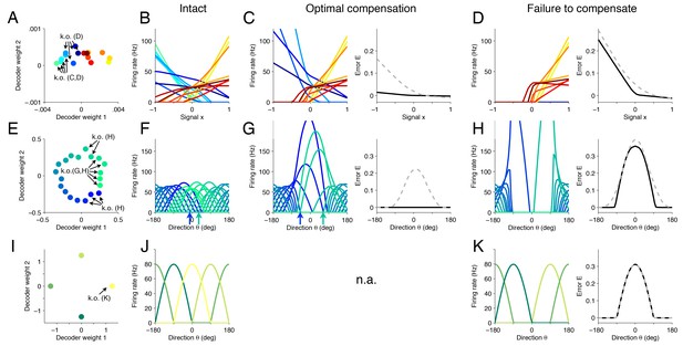
Changes in tuning curves following neuron loss and optimal compensation, as calculated with quadratic programming for three different networks.

(A) Decoding weights for a network of $N = 16$ neurons, similar to Figure 4C. Arrows indicate the neurons that will be knocked out, either in panel (C) or (D). (B) The firing rates of all neurons given as a function of the first input signal $x = x_{1}$ . Each line is the tuning curve of a single neuron, with either positive slope (yellow–red) or negative slope (blue-green). (C) Left, tuning curves after the loss of four negatively sloped neurons and after optimal compensation from the remaining neurons. Right, the signal representation continues to be accurate (black line). If the tuning curves of the remaining neurons do not undergo optimal compensation, the signal representation fails for negative values of $x$ (dashed grey line). (D) After the loss of the remaining negatively sloped neurons, the population is no longer capable of producing a readout $\hat{x}$ that can match negative values of the signal $x$ , even with optimal compensation (black line). This happens because the recovery boundary has been reached – where signal representation fails. The changes in tuning curves that occur still seek to minimize the error, as can be seen when comparing the error incurred by a network whose tuning curves do not change (dashed gray line). (E) Decoding weights for a two-dimensional network model containing $N = 20$ neurons. Apart from the smaller number of neurons and the added heterogeneity, this network is equivalent to the network shown in Figure 3. (F) This system has bell-shaped tuning curves when firing rates are plotted as a function of a circular signal with direction $θ$ . (G) Left, when some of the neurons have been knocked out, the tuning curves of the remaining neurons change by shifting towards the preferred directions of the knocked out neurons. Right, this compensation preserves high signal representation quality (black line). In comparison, if the tuning curves do not change, the readout error increases substantially (dashed gray line). (H) Left, when more neurons are knocked-out (here, all neurons with positive decoding weights), the firing rates of the remaining neurons still shift towards the missing directions (compare highlighted spike trains in Figure 3). Right, despite the compensation, the network is no longer able to properly represent the signal in all directions. (I) Decoding weights for a two-dimensional network model containing $N = 4$ neurons. (J) The network exhibits four bell-shaped tuning curves. (K) Left, following the loss of a single neuron and optimal compensation, the tuning curves of the remaining neurons do not change. Right, after cell loss, the network incurs a strong error around the preferred direction of the knocked out neuron ( $θ = 0^{o}$ ), with optimal compensation (black line) or without optimal compensation (dashed gray line).

https://doi.org/10.7554/eLife.12454.009

Figure 6

Download asset Open asset

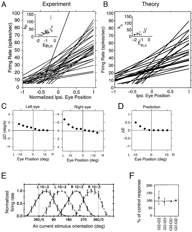
Tuning curves and inactivation experiments in the oculomotor integrator of the goldfish, and in the cricket cercal system.

(A) Tuning curve measurements from right-side oculomotor neurons (Area 1 of goldfish). Firing rate measurements above 5 Hz are fit with a straight line $f_{n} = k_{n} (x - E_{t h, n})$ , where $f_{n}$ is the firing rate of the $n^{t h}$ neuron, $E_{t h, n}$ is the firing rate threshold, $k_{n}$ is the firing rate slope and $x$ is the eye position. As the eye position increases, from left to right, a recruitment order is observed, where neuron slopes increase as the firing rate threshold increases (inset).

(B) Tuning curves from our network model. We use the same parameters as in previous figures (Figure 5A), and fit the threshold-linear model to the simulated tuning curves (Figure 5B) using the same procedure as in the experiments from Aksay et al. (2000). As in the data, a recruitment order is observed with slopes increasing as the firing threshold increases (inset). (C) Eye position drift measurements after the pharmacological inactivation of left side neurons in goldfish. Inactivation was performed using lidocaine and muscimol injections. Here $Δ D = D_{after} - D_{before}$ , where $D_{before}$ is the average drift in eye position before pharmacological inactivation and is the average drift in eye position after pharmacological inactivation. Averages are calculated across goldfish.

(D) Eye position representation error of the model network following optimal compensation. Here $Δ E = E_{C} - E_{I}$ , where is the representation error of the intact system and $E_{C}$ is the representation error following optimal compensation. These representation errors are calculated using the loss function from Equation 2 . (E) Firing rate recordings from the cricket cercal system in response to air currents from different directions. Each neuron has a preference for a different wind direction. Compare with Figure 5J.

(F) Measured change of cockroach cercal system tuning curves following the ablation of another cercal system neuron. In all cases, there is no significant change in firing rate. This is consistent with the lack of compensation in Figure 5K. The notation GI2-GI3 denotes that Giant Interneuron 2 is ablated and the change in Giant Interneuron 3 is measured. The firing rate after ablation is given as a percentage of the firing rate before ablation.

© 2000 The American Physiological Society. All Rights Reserved. Figure 6A has been adapted with permission from The American Physiological Society.

© 2007 McMillan Publisher Ltd: Nature Neuroscience. All Rights Reserved. Figure 6C has been adapted with permission from McMillan Publisher Ltd: Nature Neuroscience

© 1991 The American Physiological Society. All Rights Reserved. Figure 6E has been adapted with permission from The American Physiological Society

© 1997 The American Physiological Society. All Rights Reserved. Figure 6F has been adapted with permission from The American Physiological Society

https://doi.org/10.7554/eLife.12454.010

Figure 7

Download asset Open asset

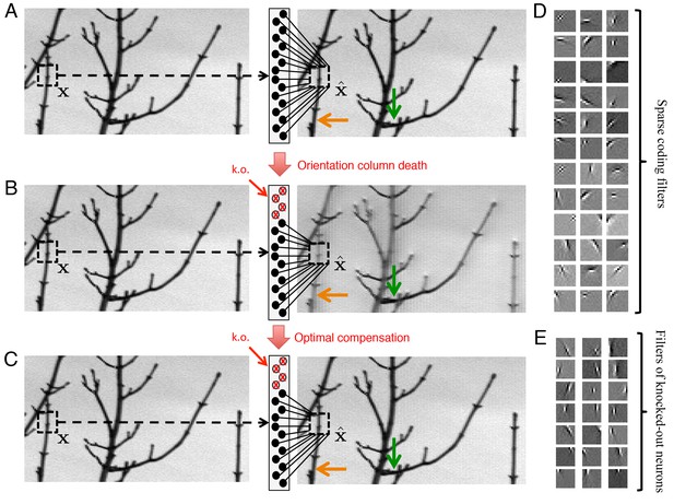
Optimal compensation for orientation column cell loss in a positive sparse coding model of the visual cortex.

(A) Schematic of a neural population (middle) providing a representation (right) of a natural image (left). This image representation is formed when neurons respond to an image patch $𝐱$ with a sparse representation and an output $\hat{x}$ . Here, patches are overlapped to remove aliasing artifacts. (B) Following the loss of neurons that represent vertical orientations, the image representation degrades substantially without optimal compensation, especially for image segments that contain vertical lines (orange arrow), and less so for image segments that contain horizontal lines (green arrow). (C) Following the optimal compensation, the image representation is recovered. (D) A selection of efficient sparse decoding weights, illustrated as image patches. Each image patch represents the decoding weights for a single neuron. In total, there are 288 neurons in the population. (E) A selection of vertically orientated decoding weights whose neurons are selected for simulated loss. All neurons with preferred vertical orientations at ${67.5}^{o}$ , $90^{o}$ and ${112.5}^{o}$ and at the opposite polarity, $- {67.5}^{o}$ , $- 90^{o}$ and $- {112.5}^{o}$ are silenced.

https://doi.org/10.7554/eLife.12454.011

Figure 8

Download asset Open asset

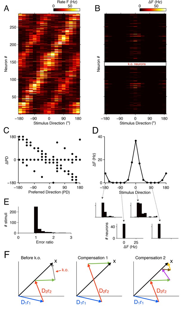
Tuning curves and signatures of optimal compensation in the V1 model.

(A) The tuning curves (firing rates as a function of stimulus direction) for all neurons in the model ( $N = 288$ ). (B) Changes in firing rates ( $Δ F$ ), as a function of stimulus direction, for all neurons in the model, when 50% of neurons with a preferred direction at $0^{\circ}$ degrees are knocked out $(N = 11)$ . Several cells change their firing close to the preferred ( $0^{\circ}$ ) or anti-preferred ( $- 180^{\circ}$ or $180^{\circ}$ ) direction of the k.o. cells. (C) The change in preferred direction, $Δ$ PD, following optimal compensation is given for each neuron as a function of its preferred direction before cell loss. Many cells shift their preferred direction towards the preferred direction of the knocked out cells. (D) The average change in firing rate due to optimal compensation ( $Δ \bar{F}$ ) is calculated at each stimulus direction, where the average is taken across the neural population in B. There is a substantial increase in firing rates close to the preferred directions of the knocked out cells. The histograms on the bottom show the firing rate changes in the population as a function of four different stimulus directions. Stimuli with horizontal orientations ( $0^{\circ}$ or $\pm 180^{\circ}$ ) lead to firing rate changes, but stimuli with vertical orientations ( $\pm 90^{\circ}$ ) do not. (E) Ratio of reconstruction errors (no compensation vs. optimal compensation) across a large range of Gabor stimuli. For most stimuli, no compensation is necessary, but for a few stimuli (mostly those showing edges with horizontal orientations) the errors are substantially reduced if the network compensates. (F) Schematic of compensation in high-dimensional spaces. In the intact state (left), a stimulus (black arrow) is represented through the firing of four neurons (colored arrows, representing the decoding vectors of the neurons, weighted by their firing rates). If the grey neuron is knocked out, one possibility to restore the representation may be to modify the firing rates of the remaining neurons (center). However, in higher-dimensional spaces, the three remaining arrows will not be sufficient to reach any stimulus position, so that this possibility is usually ruled out. Rather, additional neurons will need to be recruited (right) in order to restore the stimulus representation. These neurons may have contributed only marginally (or not at all) to the initial stimulus representation, because their contribution was too costly. In the absence of the grey neuron, however, they have become affordable. If no combination of neurons allows the system to reach the stimulus position, then the recovery boundary has been crossed.

https://doi.org/10.7554/eLife.12454.012

Figure 9 with 2 supplements

Download asset Open asset

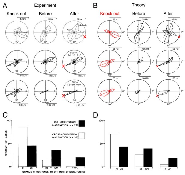
Tuning curves and inactivation experiments: Comparison between recordings from visual cortex and the V1 model.

(A) Recordings of cat visual cortex neurons both before (middle column) and after (right column) the GABA-ergic knock out of neighboring neurons (left column). The tuning curves of all neurons are shown in polar coordinates. The firing rates of all neurons increase in the direction of the preferred direction of the silenced neurons (red cross). Each row illustrates the response of a different test neuron to silencing. Examples are selected for ease of comparison with the theory. Knock-out measurements were obtained using multi-unit recording, and single-unit recordings were obtained for neurons that were not subject to silencing.

(B) A set of similarly tuned neurons are selected for the artificial knock out in our V1 model. The tuning curve of a test neuron is shown before the selected neurons are knocked out (middle column) and after optimal compensation (right column). Each row illustrates the response of a different test neuron to neuron loss. Following the optimal compensation, the neurons remaining after cell loss shift their tuning curves towards the preferred direction of the knocked out neurons (indicated by a red cross). (C) Histogram of changes in the firing rate at preferred stimulus orientations following GABA-ergic silencing. Firing rate change for neurons with tuning preferences that are similar to the recorded neurons (iso-orientation inactivation) are counted separately to changes in neurons with different tuning preferences (cross-orientation inactivation).

(D) Histogram firing rate changes in the V1 model, same format as C. In B and D we knock out $50 %$ of neurons with preferred directions across a range of $50^{o}$ (see also Figure 9—figure supplement 1).

© 1996 The American Physiological Society. All Rights Reserved. Figure 9A has been adapted with permission from The American Physiological Society

© 1992 Society of Neuroscience. All Rights Reserved. Figure 9A has been adapted with permission from Society of Neuroscience

© 1992 Society of Neuroscience. All Rights Reserved. Figure 9C is reproduced with permission from Society of Neuroscience

https://doi.org/10.7554/eLife.12454.013

Figure 9—figure supplement 1

Download asset Open asset

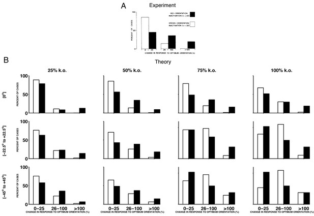
Histograms of experimental responses to neuron silencing in V1, compared to theoretical predictions using a range of different parameters.

(A) Histogram of changes in the firing rate at preferred stimulus orientations following GABA-ergic silencing. Firing rate change for neurons with tuning preferences that are similar to the recorded neurons (iso-orientation inactivation) are counted separately to changes in neurons with different tuning preferences (cross-orientation inactivation). These results are reproduced from Crook et al, 1992, see also Figure 9C. (B) Histograms of preferred compensation firing rate changes in positive sparse coding neurons, again with iso-orientation and cross-orientation neurons counted separately. Each histogram corresponds to the theoretical prediction obtained by knocking out different percentages of neurons (25%, 50%, 75% and 100%), across different ranges of preferred directions (at $0^{o}$ only, from $- {22.5}^{o}$ to ${22.5}^{o}$ , and from $- 45^{o}$ to $45^{o}$ ). We explore the full parameter space of our model, because the exact amount of neuron loss in the experiments from Crook et al (1992) is unknown. We find that when 50% or 75% of neurons with preferred directions at $0^{o}$ are knocked out, the form of the predicted histogram is similar to the experimentally recorded histogram, with a greater proportion of iso-orientation inactivations having an impact on the firing rate at the preferred stimulus orientation, compared to cross-orientation inactivation. In these calculations, we use the same sparse coding model for each histogram, with four times as many neurons as stimulus dimensions.

https://doi.org/10.7554/eLife.12454.014

Figure 9—figure supplement 2

Download asset Open asset

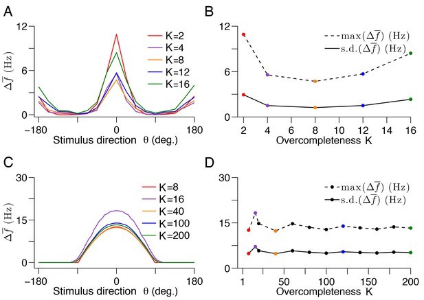
Optimal compensation in V1 models with different degrees of redundancy or over-completeness.

(A) The visual cortex contains many more neurons than input dimensions. To investigate the impact of this over-completeness, we calculate the average change in tuning curve shape following optimal compensation in our sparse coding model of V1 for increasing degrees of over completeness (see Methods). Here, the over completeness factor, $K$ is given by $K = N / M$ , where $N$ is the number of neurons and $M$ is the signal dimension. The form of the tuning curve changes is unaffected by the degree of over-completeness, but there are some fluctuations in the overall change. (B) As the degree of over completeness $K$ increases, the average change fluctuates moderately. These fluctuations are the result of inhomogeneities in our V1 model, which have a larger effect when the over-completeness factor is small. (C) Similar to A , but for the 2-d bump-shaped tuning curve model. We use the same model as before (Figure and 5E–H), but with a sparse linear cost instead of a quadratic cost. For each value of $K$ , we choose decoder weights that are evenly spaced on the unit circle. This produces evenly spaced bump-shaped tuning curves. We knock out neurons in this model and calculate the average change in tuning curve. In this case, we can easily calculate the impact of optimal compensation for systems with high degrees of over-completeness, such as the visual cortex because the dimensionality of the problem is much lower. (D) The impact of optimal compensation fluctuates moderately for low values of $K$ , as in the sparse coding model. However, as the degree of over completeness increases, the average change in tuning curve shape converges, as the fluctuations average out. The maximum and standard deviation of the average tuning curve change are calculated across all stimulus directions. In both the full sparse coding model and the 2-d model, we knock out neurons with preferred directions between $- {22.5}^{o}$ and ${22.5}^{o}$ .

https://doi.org/10.7554/eLife.12454.015

Download links

A two-part list of links to download the article, or parts of the article, in various formats.

Downloads (link to download the article as PDF)

Open citations (links to open the citations from this article in various online reference manager services)

Mendeley

Cite this article (links to download the citations from this article in formats compatible with various reference manager tools)

David GT Barrett
Sophie Denève
Christian K Machens

(2016)

Optimal compensation for neuron loss

eLife 5:e12454.

https://doi.org/10.7554/eLife.12454

Sign up for email alerts

Privacy notice