Cross-frequency synchronization connects networks of fast and slow oscillations during visual working memory maintenance
Figures
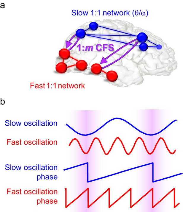
Schematic illustration of the hypothesis.
(a) Fast gamma (γ) network synchronization (red) integrates processing within the visual system while slow theta and/or alpha (θ/α) synchronization (blue) supports attentional processing in the fronto-parietal network. Cross-frequency phase synchronization (CFS) (purple) connects the fast and slow networks and regulates their communication to integrate sensory and attentional functions. (b) 1:3-phase synchronized slow (blue) and fast (red) oscillations and their phase time series. Highlights indicate how cross-frequency phase synchronization endows the fast and slow oscillation time windows where their systematic phase relationship allows spike coincidence detection and other spike-time dependent interactions to take place.
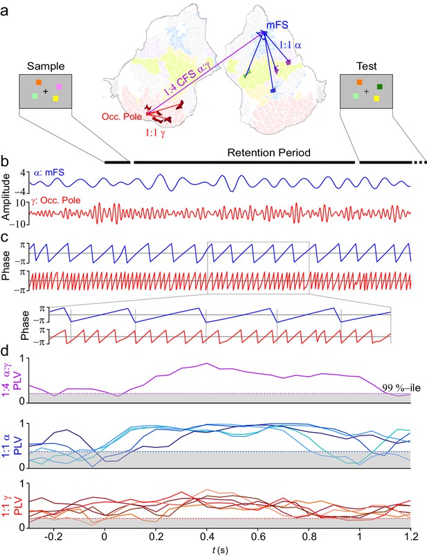
VWM modulates inter-areal cross-frequency phase synchrony (CFS) in human cortex.
Example of prominent single-trial CFS during the VWM retention period. (a) Illustration of the delayed-match-to-sample experimental paradigm where the Sample stimulus containing 1–6 colored squares is presented for 0.1 s and then after a 1 s retention period a Test stimulus appears and the subject responds whether the Test contains an object with a color different from than in Sample. The flattened cortical surface shows an example of 1:4 CFS (purple line) transiently phase coupling α (13 Hz) oscillations in the right medial frontal sulcus (MFS) with γ (54 Hz) oscillations in left occipital pole (Occ.Pole) during VWM retention. These α and γ oscillations were concurrently also 1:1 synchronized in networks of other cortical areas (blue and red lines, respectively). The cortical surface is colored by brain systems as indicated in Figure 4. (b) The signals from right MFS and left occ. pole were filtered with Morlet wavelets at 13 Hz and 54 Hz respectively. (c) The phase of the signals in (b). The zoom-in insert illustrates visually salient 1:4 cross-frequency phase synchrony during the retention period. (d) Top panel: 1:4 CFS between these α and γ oscillations was quantified with the phase-locking value (PLV) in sliding 300 ms time windows. The grey area denotes the 99%-ile confidence intervals of null hypothesis PLV values obtained with time-shifted surrogate data. CFS was strengthened during VWM retention significantly above the baseline and null hypothesis levels. Middle panel: 1:1 α phase synchrony between MFS and the five connected fronto-parietal parcels shown in (a) Bottom panel: 1:1 γ phase synchronization of Occ. Pole with the other visual cortex areas shown in (a).
-
Figure 2—source data 1
List of parcels.
List of the Destrieux-atlas parcels used in this study (see Destrieux et al., 2010 and the Freesurfer software: https://surfer.nmr.mgh.harvard.edu/).
- https://doi.org/10.7554/eLife.13451.004
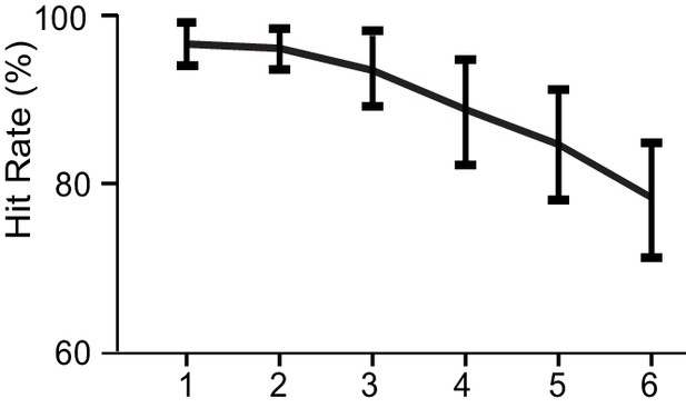
Behavioral performance.
Hit rates ± standard errors of mean (SEM) for all WVM loads.

Parcellations and subsystems.
(a) An inflated and flattened cortical surface is parcellated into 400 parcels. (b) An inflated and flattened cortical surface is parcellated into the 148 parcels of the Destrieux atlas. (c) The individual parcels are assigned to a subsystem of the Yeo parcellation.
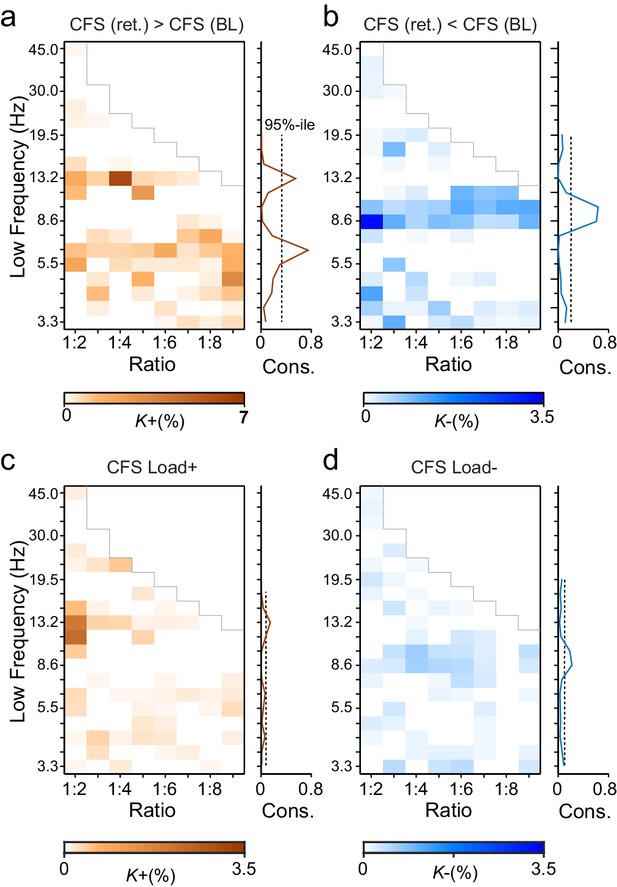
During VWM retention, inter-areal CFS was both strenghtened and suppressed in harmonic structures.
(a) Fractions (K+) of inter-areal CFS connections that were significantly stronger during VWM maintenance than in the pre-stimulus baseline (Mean condition, Wilcoxon signed ranked test, p < 0.05, corrected). K+ values (color scale) are shown for all studied pairs of 1:m ratios from 1:2 to 1:9 (x-axis) and lower frequencies from 3.3 to 45 Hz (y-axis) and represent data from an adjacency matrix for each frequency-pair. The grey line marks the boundary set by the highest investigated frequency (90 Hz). CFS of high-θ and high-α with their upper frequencies was increased for essentially all ratios. Right: The brown line indicates the harmonic consistency of CFS across low frequencies. The dashed line denotes the 95%-ile confidence limit. CFS of high-θ and high-α oscillations with their harmonics at higher frequencies is significantly consistent across ratios. (b) Fractions of inter-areal CFS connections (K-) that were suppressed below baseline levels during the retention period. Harmonic consistency (blue line) was estimated as in and shows that low-α consistent CFS was suppressed at all ratios.(c) Fractions of CFS connections that were significantly positively (K+) or (d) and negatively (K-) correlated with VWM load (Spearman Rank correlation test of CFS across the six VWM memory load conditions, p < 0.05, corrected).
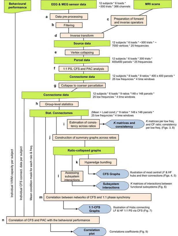
Workflow.
This Figure provides a schematic overview of the analysis steps underlying the results shown in Figures 3–9. (a) Data pre-processing, see Materials and methods: Data pre-processing. (b) Filtering into 25 frequency bands with Morlet Wavelets (see Materials and methods: Filtering). (c) Preparation of forward and inverse operators (see Materials and methods: Preparation of forward and inverse operators). (d) Inverse transform to obtain external source data (Siebenhühner et al., 2016; see Materials and methods: Inverse transform and vertex collapsing) (e) Vertex collapsing onto a parcellation of 400 brain regions. (f) 1:1 and CF synchrony analysis (see Materials and methods: 1:1 and CF synchrony analysis) (g) Collapsing onto a courser parcellation of 148 brain regions (see Materials and methods: Group-level statistics). (h) Group-level statistics to obtain the Mean and Load effect (see Materials and methods: Group-level statistics) (i) Estimation of CFS & PAC consistency across ratios (see Materials and methods: Estimation of consistency across ratios). (j) Construction of summary graphs across ratios for θ and α consistent CFS (see Materials and methods: Construction of summary graphs across ratios). (k) Bundling of edges into hyperedges to better identify true interactions from signal mixing (see Materials and methods: Bundling of edges into hyperedges). (l) Assessment of interactions between functional brain subsystems of the Yeo parcellation (see Materials and methods: Assessing interactions within and between functional brain systems). (m) Correlation between networks of CFS and 1:1 phase synchrony (see Materials and methods: Correlation between networks of CFS and 1:1 phase synchrony). (n) Correlation of subjects’ individual network strength in CFS and PAC with their behavioural performance (see Materials and methods: Correlation of CFS and PAC with the behavioral performance).
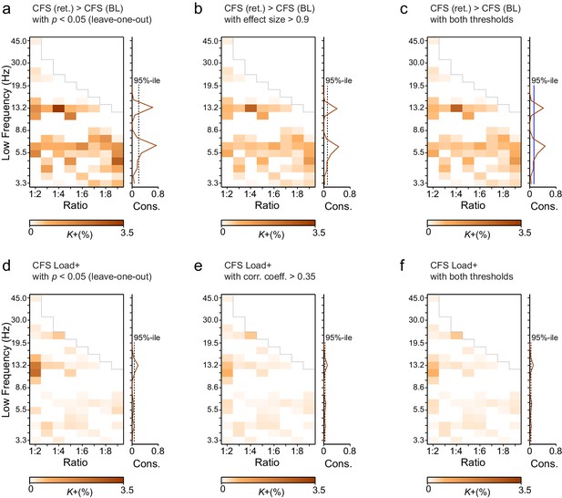
Leave-one-out statistics and effect size thresholding corroborate the robustness of CFS observations.
(a) Fractions (K+) of significant positive observations in the Mean condition (as in Figure 3 that survive thresholding with leave-one-out statistics. Here for the 12 subjects in our cohort, 12 leave-one-out cohorts of 11 subjects were created by leaving one subject out at a time. Each cohort was subjected to the same Mean condition group statistics and only those edges of the original findings (Figure 3a) were considered significant that were significant in every one of the 12 leave-one-out cohorts at the alpha level of p < 0.05. Preservation of a frequency-ratio pattern very similar to the original shows that the main findings are statistically robust and not attributable to any single subject in the cohort. (b) Fractions of significant positive observations in the Mean condition (as in Figure 3a) that also show an effect size > 0.9, which corresponds to statistical power of 0.8 or greater at N = 12. Preservation of a frequency-ratio pattern very similar to the original findings shows that the effects reported here are mostly of adequate size to be measured with the present number of subjects. (c) Fractions of edges remaining after both the leave-one-out (b) and effect size (c) thresholding. (d) Same as (a), but for the Load condition. (e) Same as (b) but for the Load condition where the effect size threshold was set to a correlation coefficient greater than 0.35. (f) As in (c), fractions of edges in original Load condition statistics that remain after combined leave-one-out (e) and effect size (f) masks.
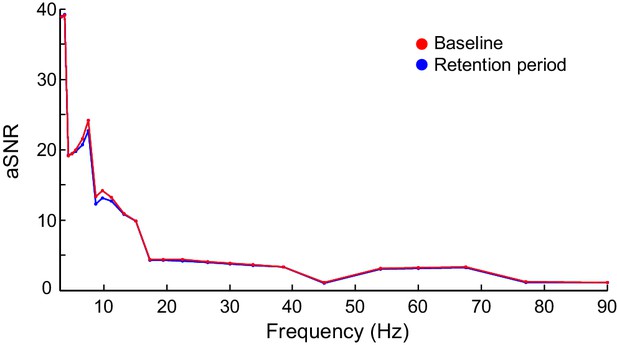
Apparent signal-to-noise ratio (aSNR) in source space.
aSNR was measured for each cortical parcel, time window, frequency band, and experimental condition as the ratio of the observed filtered signal amplitude and identically pre-processed and inverse transformed signal amplitude from empty-room MEG recordings. The figure shows Mean-condition aSNR estimates averaged across subjects and cortical parcels for the baseline (red) and the average of retention period (blue) time windows.
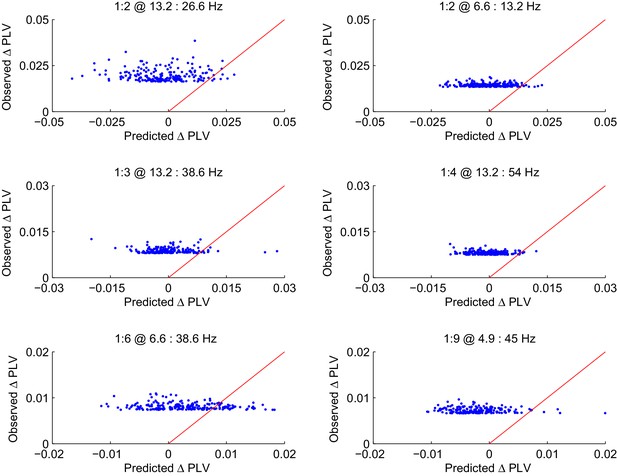
CFS PLV changes in the Mean condition are not attributable changes in the signal-to-noise ratio (SNR).
Observed changes in CFS-PLV compared against changes in PLV predicted by the local changes in SNR from the baseline to the VWM retention period. Values are shown for the 200 largest observed PLV changes for representative frequency ratios where the largest group level effects were observed. The red line represents the ideal prediction of equal values between the observed and predicted PLV. Dots left to the red line thus represent edges for which the observed PLV is greater than predicted by event-related changes in SNR.
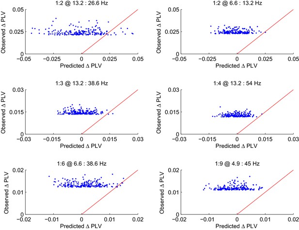
Observed PLV changes in the Load condition are not predicted by changes in SNR.
The Load condition was approximated by the difference in CFS-PLV between Load 1 and Load 6 conditions. As in Figure 3—figure supplement 4, the observed changes in this CFS-PLV difference are compared with changes in PLV that are predicted from changes in SNR from the 1 object to 6 Object condition. Values are shown for the 200 largest observed PLV changes each for the frequency ratios shown in Figure 3—figure supplement 4.
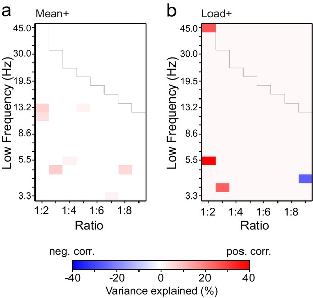
Changes in PLV and amplitude are not correlated.
(a) Variance in PLV changes that can be explained by amplitude changes in the Mean condition. Values r2∙sign(r) are shown only for ratio-frequency pairs that had K > 0.1 % in the group analysis and showed a significant correlation between PLV and amplitude effects (r) in lowest or highest 2.5% of surrogate values, N = 1000, uncorrected for multiple comparisons). (b) Same as (a), but for the Load condition.
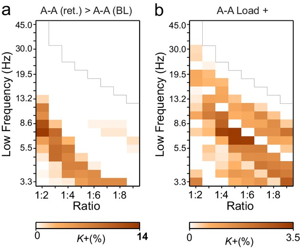
Cross-frequency (CF) amplitude-amplitude correlations do not have a low-frequency consistent harmonic structure.
(a) Fractions of edges (K+) of inter-areal CF amplitude correlations that are significantly stronger during VWM retention period than in the baseline (Mean condition, as in Figure 3a). Unlike CFS, CF amplitude correlations did not show a harmonic pattern over low frequencies. (b) Fractions of significant edges of amplitude-amplitude correlations that were positively correlated with the VWM load (Load condition, as in Figure 3c).
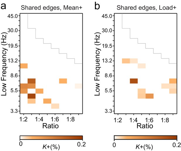
Connections with significant CFS are not co-localized with those exhibiting significant CF amplitude correlations.
Fractions of edges, K, which were significant in (a) Mean- and (b) Load-conditions in both the CFS and CF-amplitude correlation analyses. Compared to the original networks (see Figure 3a,c and Figure 3—figure supplement 6) these very low K values show that there is little neuroanatomical co-localization in the networks of CFS and CF amplitude correlations.
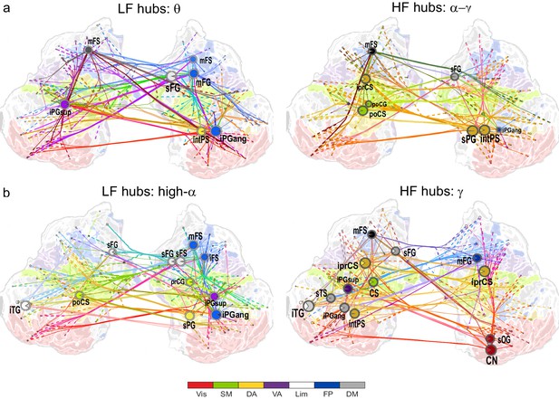
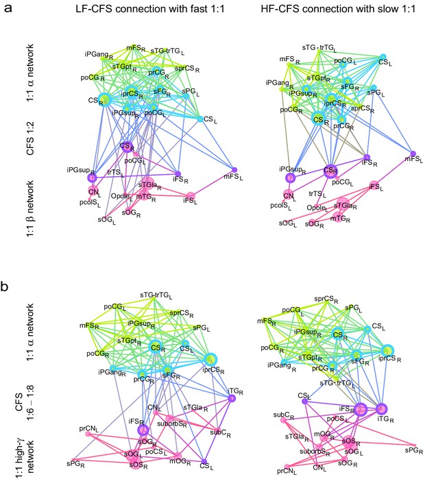
θ- and high-α-consistent CFS is observed in fronto-parietal and visual networks.
(a) Low-frequency CFS hubs (LF, left) and high-frequency CFS hubs (HF, right) and their most central connections during the VWM retention period for θ-consistent CFS averaged across memory loads (Mean condition) and shared across frequency ratios from 1:2−1:9 (see Materials and methods for details) displayed on a flattened cortical surface. These networks and the most central low- and high-frequency hubs are presented here separately to illustrate the distinct neuroanatomical sources of the most central cortical θ oscillations (left) and the α−γ oscillations (right) connected by this CFS coupling. The complete θ-consistent CFS network is thus the combination of these graphs. Circles represent network vertices (cortical parcels), their size is proportional to their degree centrality, and both vertex and surface colors represent functional brain systems (see colors below). The lighter sector of each vertex represents the fraction of low-frequency connections and the darker section the fraction of high-frequency connections this vertex has in the graph. The width of the edges represents the coupling strength between the two vertices and their color is a mixture of the brain system assignments of the vertices. The dotted lines at the end of the connections point towards the high-frequency (from LF hubs, left panel) or the low-frequency (from HF hubs, right panel) vertices for LF and HF networks, respectively. (b) As in (a), but for the high-α-consistent CFS shared across ratios from 1:3−1:9. Functional subsystem abbreviations: Vis: Visual, SM: Sensorimotor, DA: Dorsal Attention, VA: Ventral Attention, Lim: Limbic, FP: Frontoparietal, DM: Default Mode.
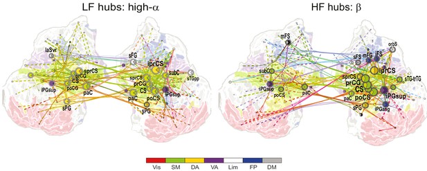
1:2 CFS between high-α and β bands is most pronounced in the sensorimotor network.
Low-frequency (LF, left) and high-frequency (HF, right) hubs and their connections for CFS between high-α and β frequencies at ratio 1:2 in the Mean condition (all illustration details as in Figure 4a).
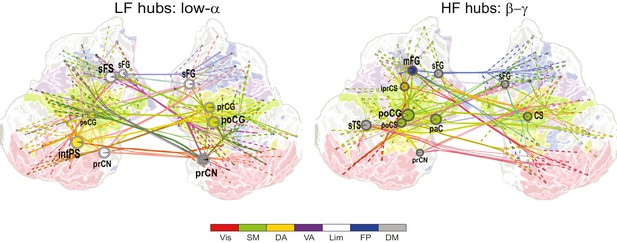
Network of low-α consistent CFS suppression.
Low-frequency (LF, left) and high-frequency (HF, right) hubs and their connections for low-α consistent CFS suppression during VWM retention period averaged across memory loads (Mean condition) and shared across ratios from 1:2−1:9 (all illustration details as in Figure 4a).
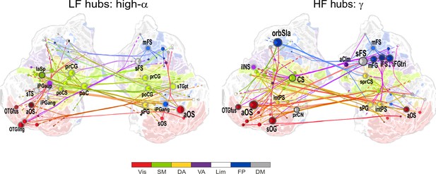
1:3−1:9 CFS between high-α and γ oscillations is VWM load-dependently strengthened among visual, sensorimotor, and frontoparietal networks during the retention period.
Low-frequency high-α (LF, left) and corresponding high-frequency γ (HF, right) CFS hubs and their connections for the Load condition high-α-consistent CFS shared across ratios 1:3−1:9 (all illustration details as in Figure 4a).
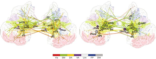
VWM-load-dependent strengthening of 1:2 CFS between high-α and β oscillations is observed in largely in sensorimotor, but also in attentional brain systems.
Low-frequency (LF, left) and high-frequency (HF, right) CFS hubs and their connections for significant positive correlations with VWM memory load (Load condition) for CFS between high-α and β frequencies at ratio 1:2 (as in Figure 5, all illustration details as in Figure 4a).
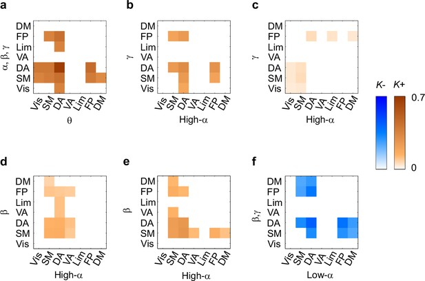
CFS connects task-relevant functional brain systems.
(a) Connection density K for θ consistent CFS (ratios 1:2–1:9) in the Mean condition within and between functional brain systems of the Yeo parcellation. The x-axis shows the subsystems for the lower frequency and the y-axis for the higher frequency oscillations. K is shown for those brain system pairs where K exceeded the 95%-ile of the corresponding K values obtained with surrogate data. (b,c) Same as (a), but for high-α consistent CFS (ratios 1:3–1:9) in the Mean and Load conditions, respectively. (d,e) Same as (a), but for α:β CFS (ratio 1:2) in the Mean and Load conditions, respectively. (f) K of low-α consistent CFS decreases (negative Mean condition) within and between systems.
-
Figure 6—source data 1
Statistical table for connection densities.
Connection density K of significant CFS connections within and between functional brain systems and 95th percentile for K from 5000 randomized surrogate graphs. The low-frequency subsystems are given in rows and the high-frequency subsystems in columns. Vis=Visual, SM=sensorimotor, DA=dorsal attention, VA=ventral attention, Lim=Limbic, FP=frontoparietal, DM=default mode
- https://doi.org/10.7554/eLife.13451.022
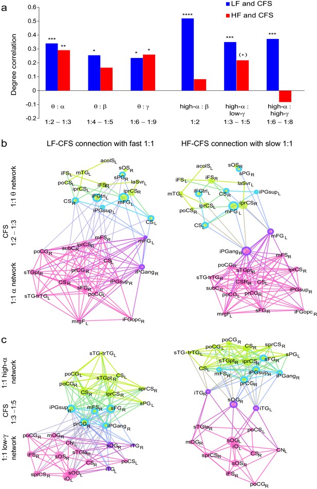
CFS connects the hubs of the low- and high-frequency 1:1 phase synchronized networks.
(a) Correlation of vertex degree centrality values of the low- (blue) and high- (red) frequency CFS network vertices with the vertices of 1:1 phase synchronized networks in the same frequency bands (Pearson correlation test, ***p < 0.001; **p < 0.01; *p < 0.05; (*) p < 0.05 uncorrected. The p values, save for (*), are corrected for multiple comparisons with Benjamini-Hochberg FDR method). (b) Simplified illustration of CFS connecting 1:1 networks. The graph shows 15 brain areas with the greatest degree centrality in significantly 1:1 phase synchronized (Mean-condition) θ-band (green) and α-band networks (pink). Blue borders indicate the brain areas that belong to the most central low-frequency CFS-hubs while the violet borders indicate the brain areas that are among the most central high-frequency CFS hubs. Significant CFS coupling between these networks is shown in a separated manner for clarity: left column shows CFS coupling of the low-frequency CFS hubs with all of their targets in the 1:1 higher-frequency network. Conversely, the right column shows the CFS coupling of the high-frequency CFS hubs with all of their targets in the 1:1 lower-frequency network. Individual brain areas may appear both as low- and high-frequency hubs within the same graph. (c) CFS coupling between 1:1 high-α-band network (green) and the low-γ-band network (pink). All visualization details as in (b).
-
Figure 7—source data 1
Statistical table for correlation coefficients r and p-values.
Statistical r and p values for the correlation between vertex degree values of the LF and HF CFS hubs with the corresponding hubs of the within-frequency synchronized networks estimated with Pearson´s correlation test. Values are corrected for multiple comparisons by Benjamini-Hochberg FDR method. Correlations with p < 0.05 are marked in green when significant after correction for multiple comparisons with Benjamini-Hochberg or yellow if not significant after correction.
- https://doi.org/10.7554/eLife.13451.024
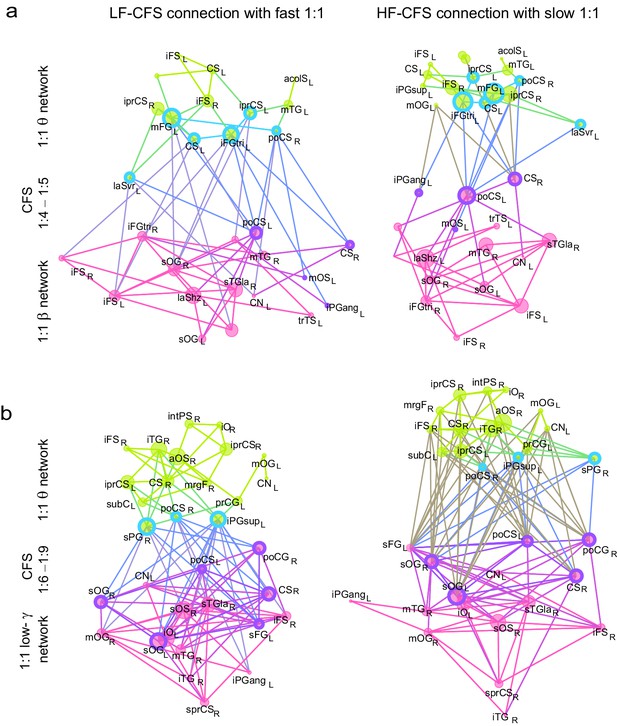
CFS connects the hubs of 1:1 synchronized networks in θ and β-γ bands.
(a, b) Simplified illustration of θ:β CFS connecting θ and β 1:1 networks, see Figure 7 for details.
CFS connects the hubs of 1:1 synchronized networks in α and β−high-γ bands.
(a, b) Simplified illustration of high-α:high-γ CFS connecting 1:1 high-α and high-γ networks, see Figure 7 for details.
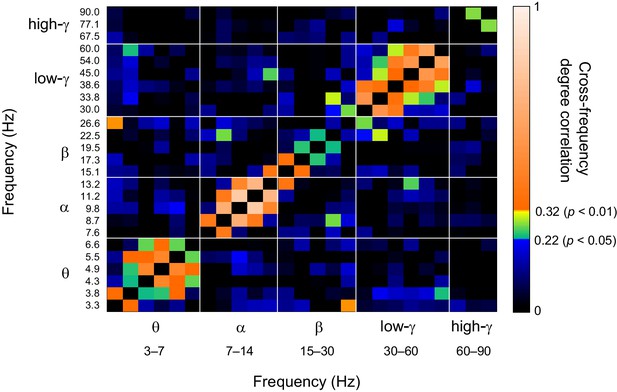
Network vertex centralities are correlated among oscillations with nearby frequencies.
Similarity of parcel degrees among significant Mean-condition 1:1 phase synchronization networks for all frequencies analysed in this study. Similarity was estimated with the Pearson correlation coefficient of vertex degrees. Color scale segments indicate p < 0.05 or p < 0.01 (uncorrected) to index the reliability of the correlations.
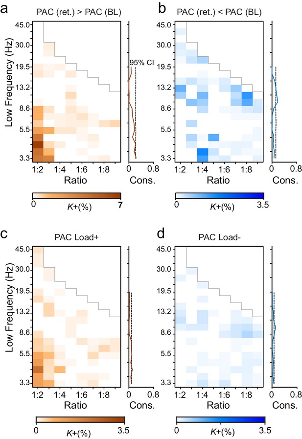
Phase-amplitude coupling (PAC) couples the phases of low-frequency θ and α oscillations with the amplitudes of faster α–γ oscillations.
(a) Fractions of strengthened (K+) and (b) suppressed (K-) PAC in the Mean condition. PAC couples the phase of the low-frequency (y-axis) oscillations with the amplitudes of the faster oscillations at the frequency ratio on the x-axis. The harmonic consistency for PAC is shown on the right as in Figure 3a and b for CFS. PAC was suppressed below baseline levels for the high-α consistent ratios where CFS was strengthened and did not show significant harmonic consistency. (c) Load-dependent increases and (d) decreases in PAC (comparable with the Load condition CFS in Figure 3c and d).
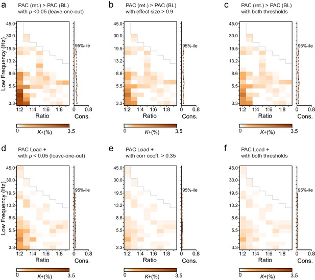
Leave-one-out statistics and effect size thresholding corroborate also the robustness of PAC observations.
(a and d) Leave-one-out statistical thresholding of the original PAC findings in Figure 8 in the Mean and Load conditions (all procedures for these figures are identical to those used for CFS; for details, see Figure 3—figure supplement 2). (b and e) Effect-size thresholding of the original PAC findings in Figure 8 in the Mean and Load conditions. (c and f) Combined leave-one-out statistics and effect-size thresholding of the original PAC findings in Figure 8 in the Mean and Load conditions.
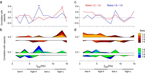
The strength of CFS predicts individual VWM capacity.
(a) Correlation of subjects’ individual CFS network strength in the Mean condition with their behavioral VWM capacity for low (1:2−1:5, red line) or high (1:6−1:9, blue line) ratios. Positive correlation is found for low ratios in the high-α band and for high ratios in the θ band (Pearson correlation, **p < 0.01 after correction for multiple comparisons with the Benjamini-Hochberg method). (b) Correlation coefficients of subjects’ individual CFS network strength with their VWM capacity for each ratio are shown cumulatively to illustrate the systematic correlation across ratios at high-α and θ frequencies. For the ratio colors, see legend in (d). Upward correlations indicate positive correlations with capacity and downward ones negative correlations. (c) Correlation of subjects’ individual PAC network strength with their VWM capacity, visualized as in (a). (d) Correlation of subjects’ individual PAC network strength with their VWM capacity for individual ratios, visualized as in (b).
-
Figure 9—source data 1
Statistical Table for the correlation of CFS and PAC values with the individual VWM capacity.
Pearson´s correlation coefficients r and p values for the correlation of CFS and PAC network strength with subject's individual VWM capacity. Correlations with p < 0.05 are marked in green when significant after correction for multiple comparisons with Benjamini-Hochberg or yellow if not significant after correction.
- https://doi.org/10.7554/eLife.13451.031
-
Figure 9—source data 2
Statistical Table for the correlation of CFS and PAC values with the individual VWM capacity.
Positive and negative correlations in individual ratios are given by Pearson´s correlation coefficient r.
- https://doi.org/10.7554/eLife.13451.032


