The modulation of savouring by prediction error and its effects on choice
- University College London, United Kingdom
- Max Planck UCL Centre for Computational Psychiatry and Ageing Research, United Kingdom
Figures
Figure 1
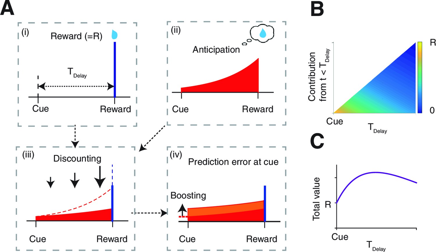
The model.
(A) The value of the cue is determined by (ii) the anticipation of upcoming reward in addition to (i) the reward itself. The two are (iii) linearly combined and discounted; with the weight of anticipation being (iv) boosted by the RPE associated with the predicting cue. (B) The contribution of different time points to the value of predicting cue. The horizontal axis shows the time of reward delivery. The vertical axis shows the contribution of different time points to the value of the predicting cue. (C) The total value of the predicting cue, which integrates the contribution along the vertical axis of panel (B), shows an inverted U-shape.
Figure 2 with 2 supplements
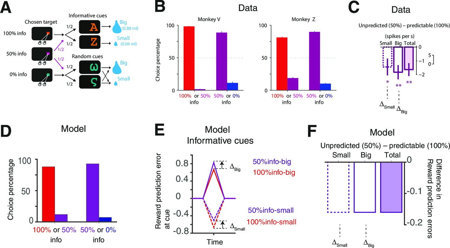
Our model accounts for the behavioral and neural findings in Bromberg-Martin and Hikosaka (2011).
(A) The task in (Bromberg-Martin and Hikosaka, 2011). On each trial, monkeys viewed a fixation point, used a saccadic eye movement to choose a colored visual target, viewed a visual cue, and received a big or small water reward. The three potential targets led to informative cues with 100%, 50% or 0% probability. (Bromberg-Martin and Hikosaka, 2011; reproduced with permission) (B) Monkeys strongly preferred to choose the target that led to a higher probability of viewing informative cues (Bromberg-Martin and Hikosaka, 2011; reproduced with permission). (C) The activity of lateral habenula neurons at the predicting cues following the 100% target (predictable) were different from the case where the cues followed the 50% target (unpredicted) (Bromberg-Martin and Hikosaka, 2011; reproduced with permission). The mean difference in firing rate between unpredicted and predictable cues are shown in case of small-reward and big-reward (the error bars indicate SEM.). (D) Our model predicts the preference for more informative targets. (E,F) Our model’s RPE, which includes the anticipation of rewards, can account for the neural activity. Note the activity of the lateral habenula neurons is negatively correlated with RPE.
Figure 2—figure supplement 1
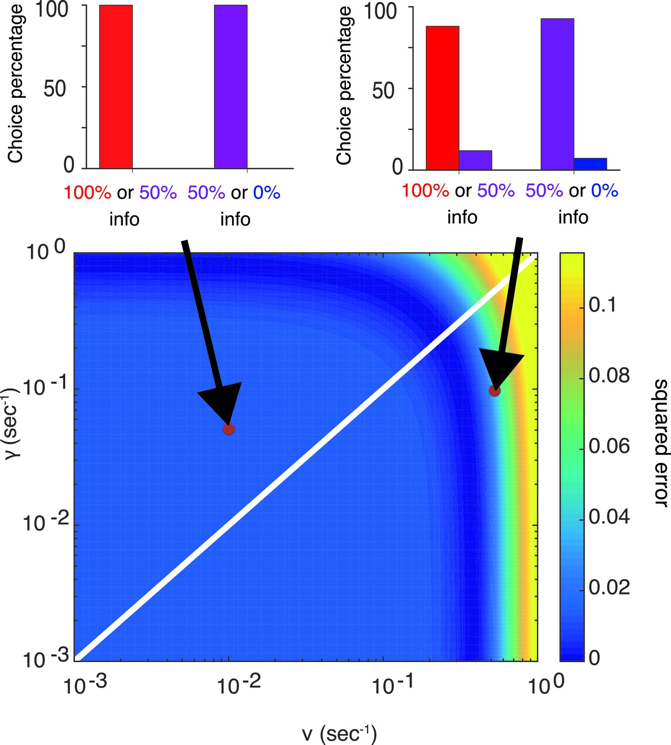
Our model can capture the preference of info targets with a wide range of parameters.
The color map (bottom) shows the squared errors of our model’s prediction with respect to the choice preference of one of the monkeys (Monkey Z) reported in Bromberg-Martin and Hikosaka (2011), while the top two panels show model’s predictions the corresponding parameters. The parameters are fixed, not optimized, as
Figure 2—figure supplement 2
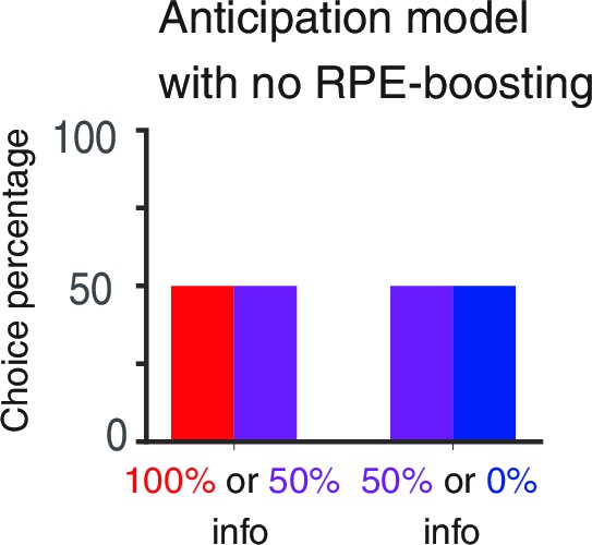
RPE-boosting of anticipation is necessary to capture the choice preference of monkeys reported in Bromberg-Martin and Hikosaka (2011).
The baseline anticipation is the same for three targets with different levels of advance reward information. Hence the model exhibits no preference.
Figure 3 with 2 supplements
Our model accounts for a wide range of seemingly paradoxical findings of observing and information-seeking.
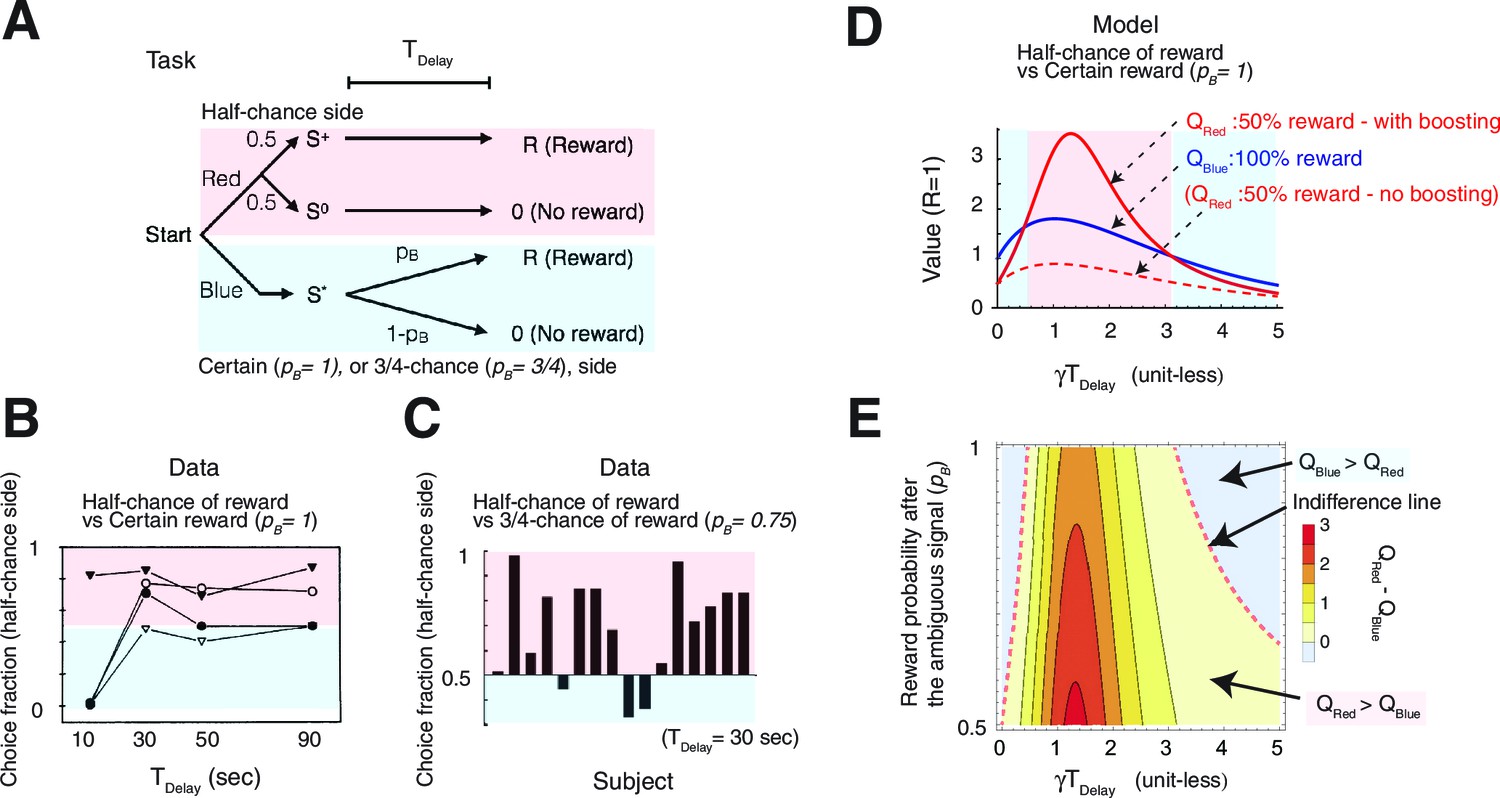
(A) Abstraction of the pigeon tasks reported in Spetch et al. (1990); Gipson et al. 2009). On each trial, subjects chose either of two colored targets (Red or Blue in this example). Given Red, cue or was presented, each with probability 0.5; was followed by a reward after time , while was not followed by reward. Given Blue, a cue was presented, and reward possibly followed after the fixed time delay with probability pB, or otherwise nothing. In Spetch et al. (1990), pB=1, and in Gipson et al. (2009) pB=0.75. (B) Results with pB=1 in Spetch et al. (1990). Animals showed an increased preference for the less rewarding target (Red) as delay time was increased. The results of four animals are shown. (Adapted from Spetch et al., 1990) (C) Results with pB=0.75 in Gipson et al. (2009). Most animals preferred the informative but less rewarding target (Red). (Adapted from Gipson et al., 2009) (D) Our model predicted changes in the values of cues when pB=1, accounting for (B). Thanks to the contribution of anticipation of rewards, both values first increase as the delay increased. Even though choosing Red provides fewer rewards, the prediction error boosts anticipation and hence the value of Red (solid red line), which eventually exceeds the value of Blue (solid blue line), given a suitably long delay. Without boosting, this does not happen (dotted red line). At the delay gets longer still, the values decay and the preference is reversed due to discounting. This second preference reversal is our model’s novel prediction. Note that x-axis is unit-less and scaled by . (E) The changes in the values of Red and Blue targets across different probability conditions pB. Our model predicted the reversal of preference across different probability conditions of pB. The dotted red line represents when the target values were equal. We set parameters as .
Figure 3—figure supplement 1

Related to Figure 3.
The changes in the values of Red and Blue targets across different probability conditions when we assume a different function form for (the task described in Figure 3). The model’s behavior does not change qualitatively compared to Figure 3D;E. We set parameters as .
Figure 3—figure supplement 2
Related to Figure 3.
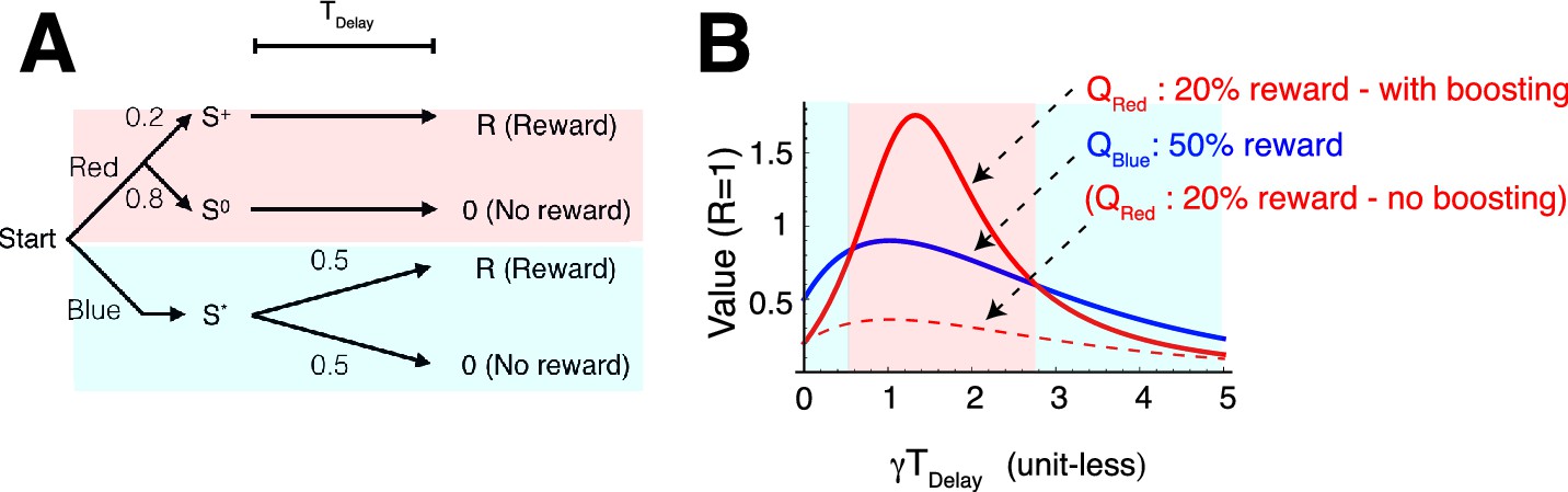
(A) The task reported in Stagner and Zentall (2010); Vasconcelos et al. (2015); Zentall (2016). Subjects (birds) had to choose either the 100% info target (shown as Red here) associated with 20% chance of reward, or the 0% info target (shown as Blue here) associated with 50% chance of reward. Subjects preferred less rewarding Red target. (B) Our model accounts for the data. Because of the boosted anticipation of rewards, the model predicted a preference of less rewarding, but informative, Red target at finite delay periods . Without boosting, the model predicts a preference of Blue over Red at any delay conditions. Model parameters were taken as the same as Figure 3: .
Figure 4 with 2 supplements
Human decision-making Experiment-1.
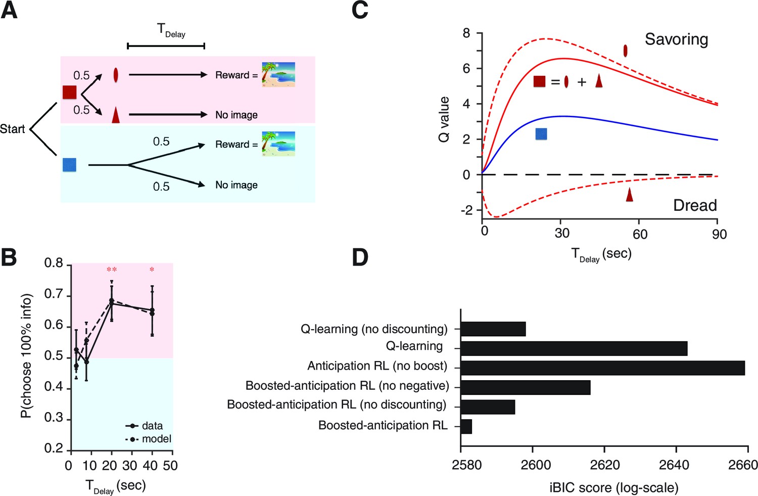
(A) On each trial, subjects chose either of two colored targets (Red or Blue in this example). Given Red, cue (oval) or (triangle) was presented, each with probability ; was followed by a reward (an erotic picture) after time , while was not followed by reward. Given Blue, either a reward or nothing followed after the fixed time delay with probability each. (B) Results. Human participants (n=14) showed a significant modulation of choice over delay conditions [one-way ANOVA, F(3,52)=3.09, p=0.035]. They showed a significant preference for the 100% info target (Red) for the case of long delays [20 s: , , 40 s: , ]. The mean +/- SEM indicated by the solid line. The dotted line shows simulated data using the fitted parameters. (C) Mean Q-values of targets and predicting cues estimated by the model. The value of informative cue is the mean of the reward predictive cue (oval), which has an inverted U-shape due to positive anticipation, and the no-reward predictive cue (triangle), which has the opposite U-shape due to negative anticipation. The positive anticipation peaks at around 25 s, which is consistent with animal studies shown in Figure 3(B,C). See Table 2 for the estimated model parameters. (D) Model comparison based on integrated Bayesian Information Criterion (iBIC) scores. The lower the score, the more favorable the model. Our model of RPE-boosted anticipation with a negative value for no-outcome enjoys significantly better score than the one without a negative value, the one without RPE-boosting, the one without temporal discounting, or other conventional Q-learning models with or without discounting.
Figure 4—figure supplement 1
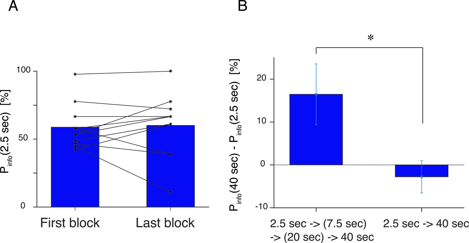
(A) Control experiment, where the first block and the last (5th) block of the experiment had the same delay duration of s.
Subjects showed no difference [, ] in the preference before and after experiencing the other delay conditions. (B) The large change in the delay duration affects on choice behavior. Y-axis shows the difference in choice percentage between the shortest (2.5 s) and the longest (40s) delay conditions. In our main experiment, the delay duration was gradually increased (Left), while in the control experiment, the delay was abruptly increased. The difference between the two procesures was significant [2 sample , ]. Subjects reported particularly unpleasant feeling for the long delay condition in the control experiment.
Figure 4—figure supplement 2
The generated choice by the model without the negative value assigned to the no-reward outcome.
The model fails to capture the short delay period (7.5 s). This corresponds to the time point at which the the effect of negative anticipation was the largest, according to the model with .
Figure 5
Human decision-making Experiment-2.
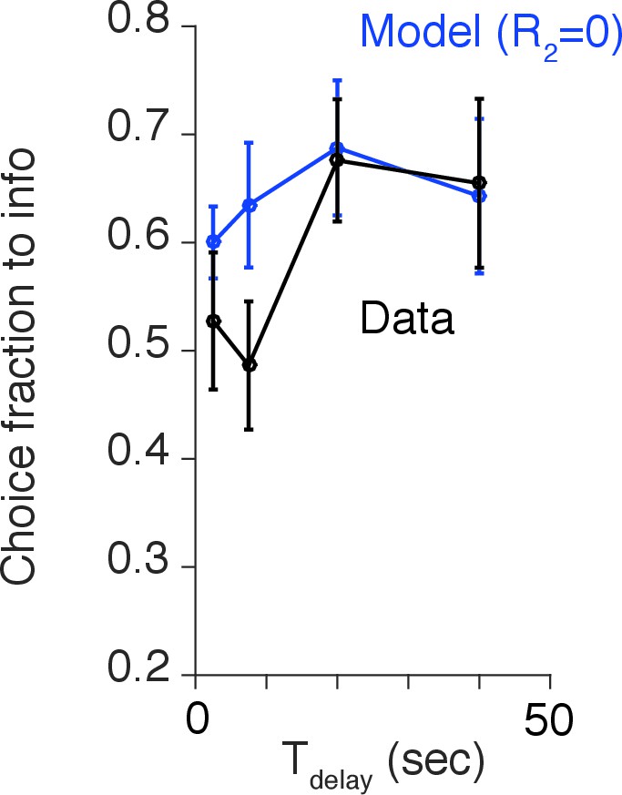
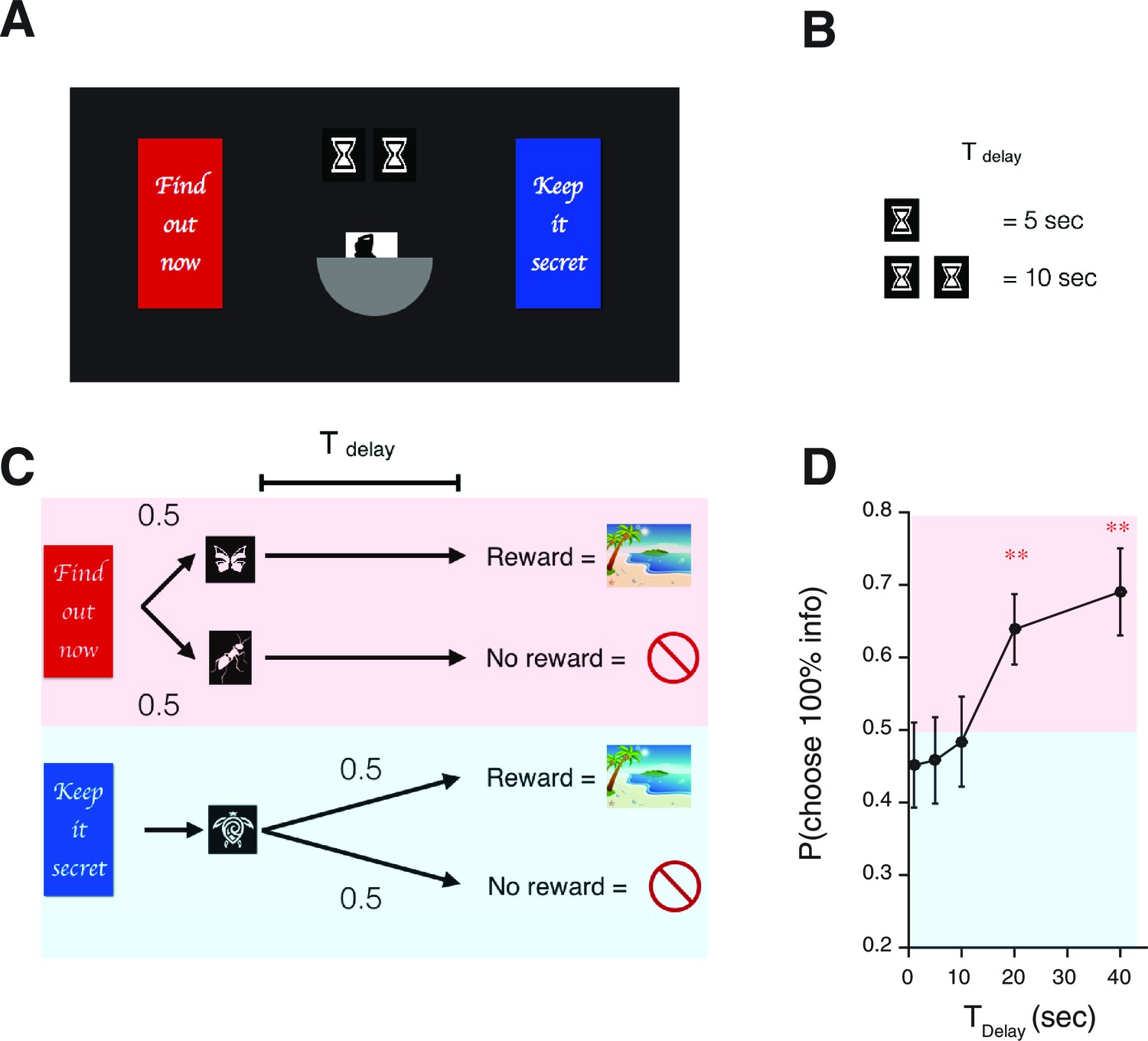
(A) A screen-shot from the beginning of each trial. The meaning of targets ('Find out now' or 'Keep it secret'), the duration of (the number of hourglass), and the chance of rewards (the hemisphere ) were indicated explicitly. (B) The number of hourglasses indicated the duration of until reward. One hourglass indicated 5 s of . When s, a fraction of an hourglass was shown. This was instructed before the experiment began. The delay condition was changed randomly across trials. (C) The task structure. The task structure was similar to Experiment-1, except that the 0% info target (Blue) was followed by a no-info cue, and an image symbolizing the lack of reward was presented when no reward outcome was delivered. (D) Results. Human participants (n=31) showed a significant modulation of choice over delay conditions [one-way ANOVA, F(4,150)=3.72, p=0.0065]. The choice fraction was not different from 0.5 at short delays [1 s: , 5 s: , , 10 s: , ] but it was significantly different from 0.5 at long delays [20 s: , , 40 s: , ], confirming our model’s key prediction. The mean and +/- SEM are indicated by the point and error bar.
Tables
Table 1
iBIC scores. Related to Figure 4.
| Model | N of parameters | Parameters | iBIC |
|---|---|---|---|
| Q-learning (with no discounting) | 3 | ,, | 2598 |
| Q-learning (with discounting) | 5 | ,,,, | 2643 |
| Anticipation RL without RPE-boosting | 7 | , , , , , , | 2659 |
| Boosted anticipation RL without | 4 | , ,, | 2616 |
| Boosted anticipation RL with no discounting | 5 | , , , , | 2595 |
| Boosted anticipation RL | 6 | , , , , , | 2583 |
Table 2
Related to Figure 4. The group means that estimated by hierarchical Bayesian analysis for our human experiment.
| 0.17 | 0.85 | -0.84 | 0.041 () | 0.082 () | 0.41 () |
Download links
A two-part list of links to download the article, or parts of the article, in various formats.
Downloads (link to download the article as PDF)
Open citations (links to open the citations from this article in various online reference manager services)
Cite this article (links to download the citations from this article in formats compatible with various reference manager tools)
The modulation of savouring by prediction error and its effects on choice
eLife 5:e13747.
https://doi.org/10.7554/eLife.13747


