Spontaneous mutations and the origin and maintenance of quantitative genetic variation
- North Carolina State University, United States
- Knox College, United States
Figures
Figure 1
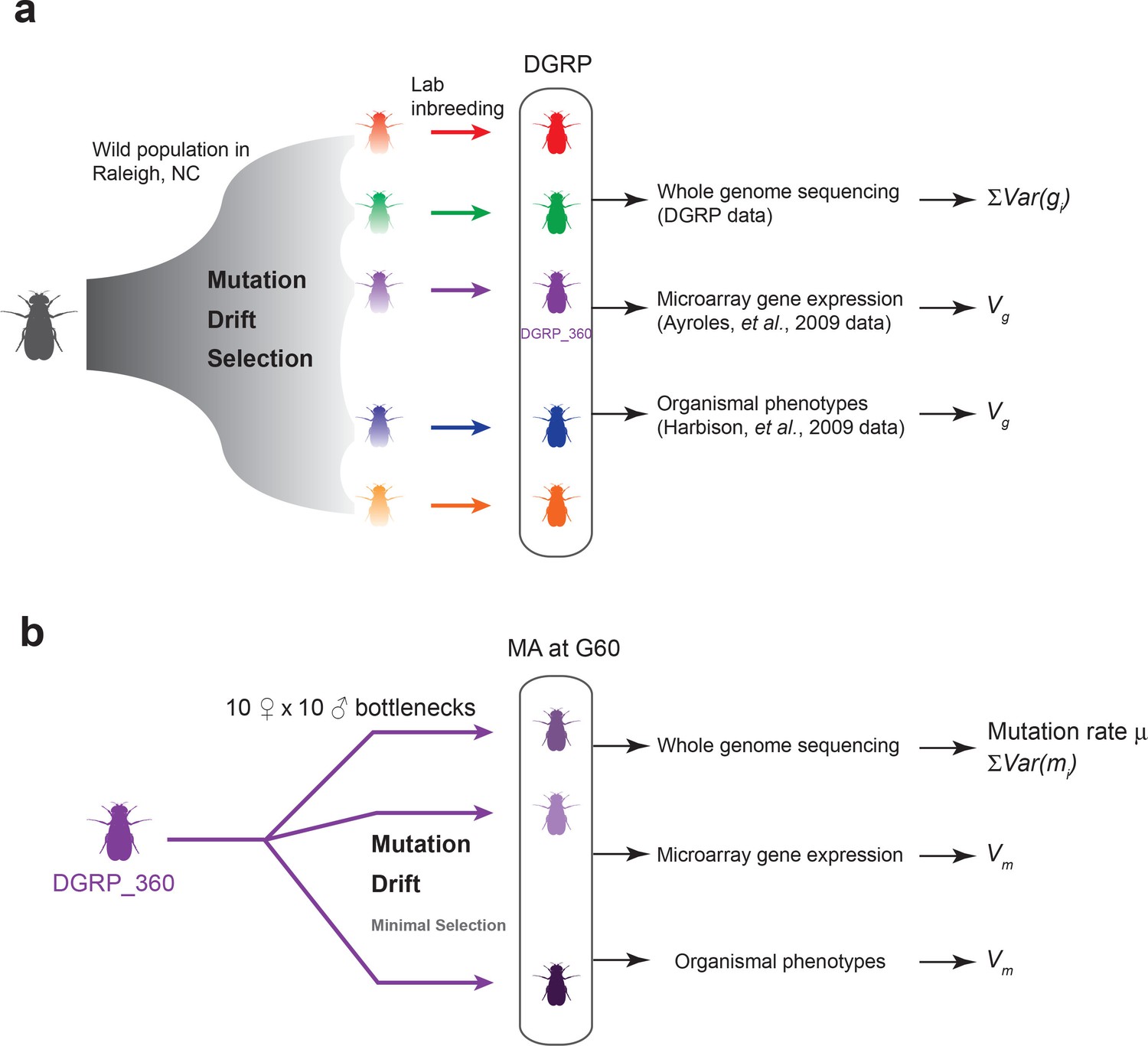
Experimental design of the DGRP and mutation accumulation (MA) lines.
(a) The DGRP is a collection of inbred strains derived from the wild population in Raleigh, NC. The spectrum of mutations and genetic variation in the DGRP is a reflection of the combined effects of mutations, drift, and selection. In this study, we used the DGRP genotype data (Huang et al., 2014) to estimate the parameter (see Materials and methods), the microarray expression data collected by (Ayroles et al., 2009) and organismal phenotypes (sleep traits from Harbison et al., 2009) to estimate genetic variance among the DGRP lines (). (b) We derived 25 MA lines from the inbred line DGRP_360. These lines were kept with small population sizes of 10 females and 10 males such that there is minimal natural selection. At generation 60, we sequenced the MA lines to estimate mutation rate () and , and obtained microarray gene expression and organismal phenotypic data to estimate mutational variance ().
Figure 2
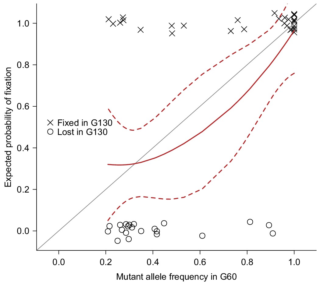
Validation of mutations.
51 Mutations detected at G60 (frequency > 0.2) in MA lines 2, 11, 13, 17, or 24 were randomly selected and sequenced by Sanger sequencing at G130 and classified as Fixed (cross) or Lost (circle) by manually inspecting chromatograms. The fixation status is plotted against the initial mutant frequency at G60. A LOESS smooth line was fitted to the data (point estimates = solid line, 95% confidence interval = broken line) to estimate the fixation probability. Expectation of fixation probability (= initial mutant allele frequency) is indicated by the grey diagonal line.
Figure 3
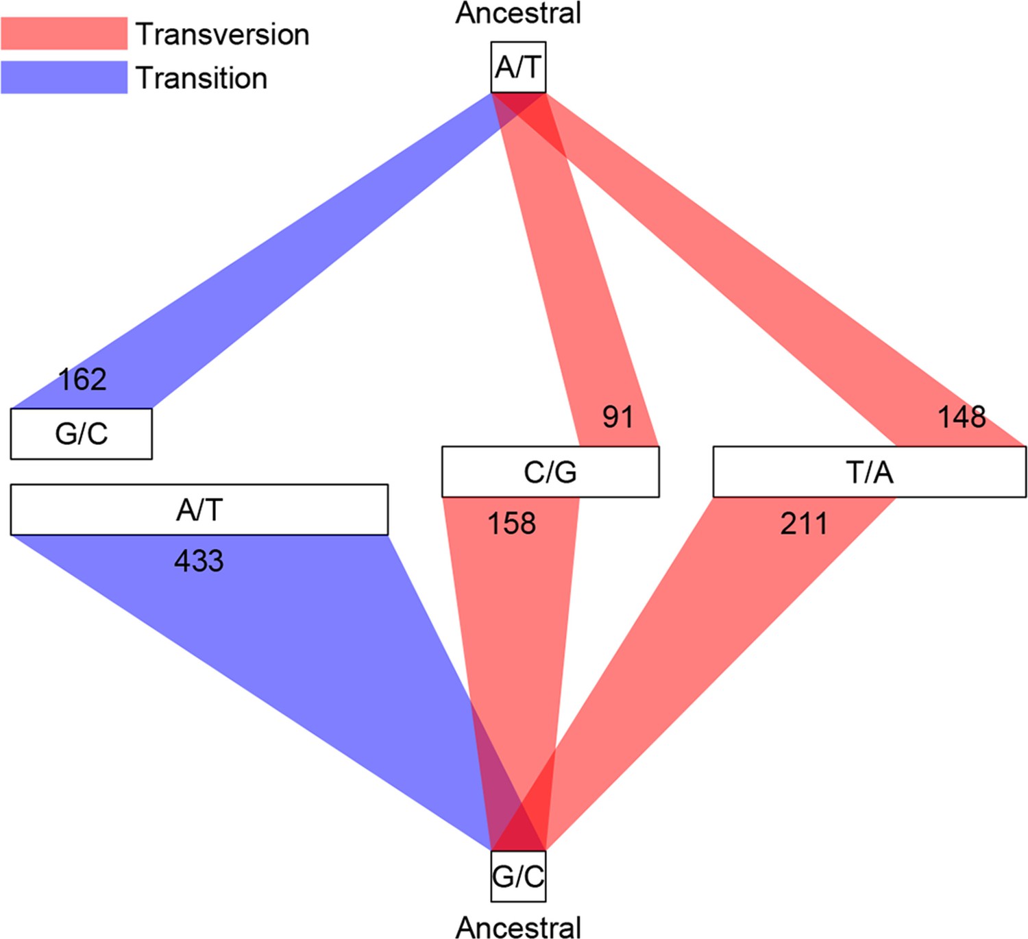
Classification of single base substitutions (SBS).
Single base substitutions were classified according to their ancestral alleles (top and bottom box) and mutant alleles (middle boxes). The size of each of the middle boxes indicates number of mutations in each class. Blue and red lines indicate transitions and transversions, respectively.
Figure 4
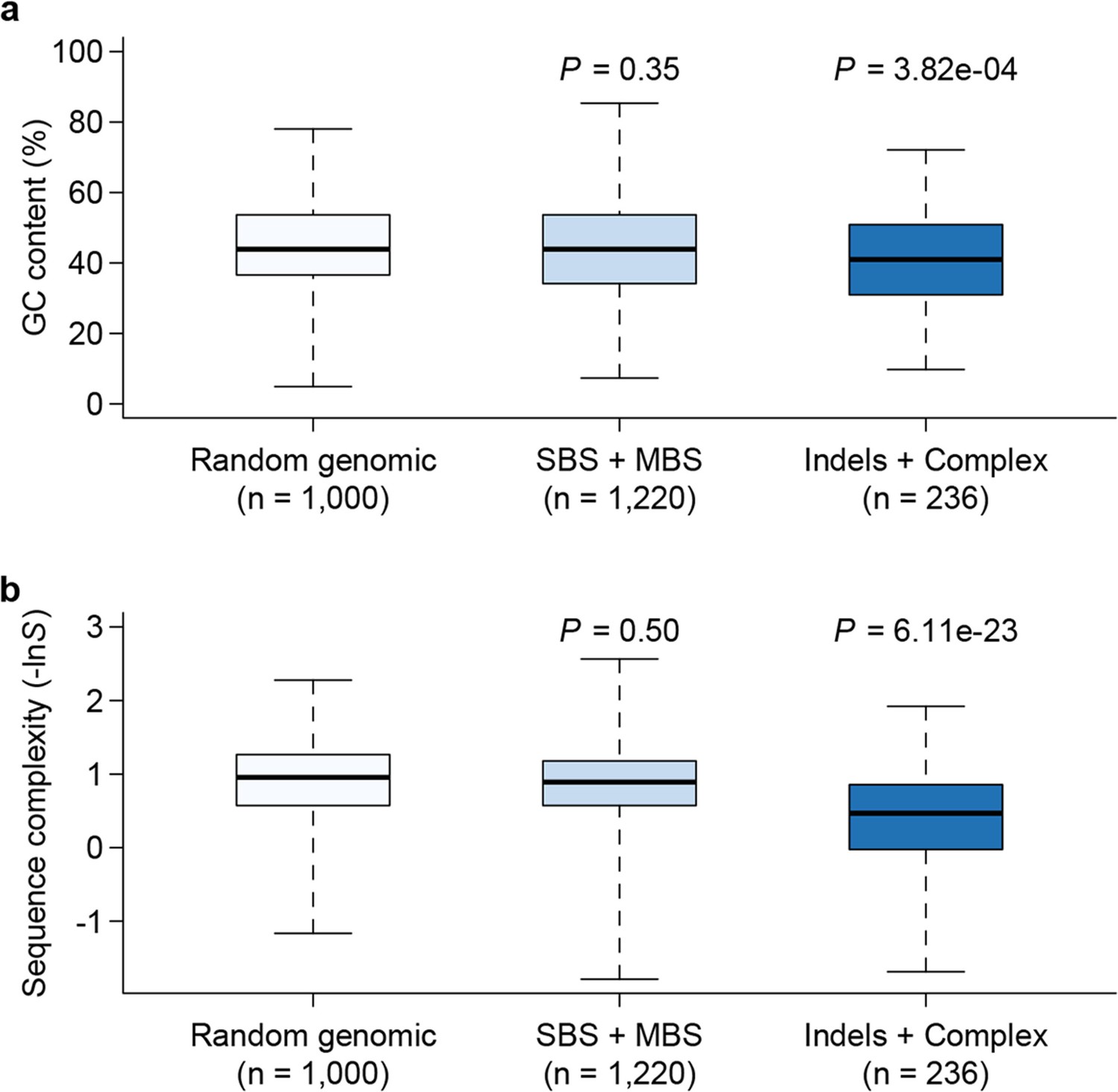
Genomic context of mutations.
Sequence composition (GC content, a) and complexity (b) for local sequences (20 bp up and downstream of mutations) are plotted as box plots and compared between different types of mutations. The 'Random genomic' class contains 1000 randomly chosen sites in the genome. Sequence complexity is measured as –lnS, where S is calculated using the algorithm in NCBI’s DUST program and measures sequence complexity. P values were computed by Wilcoxon’s rank sum tests comparing data in each category to the 'Random genomic' category.
Figure 5
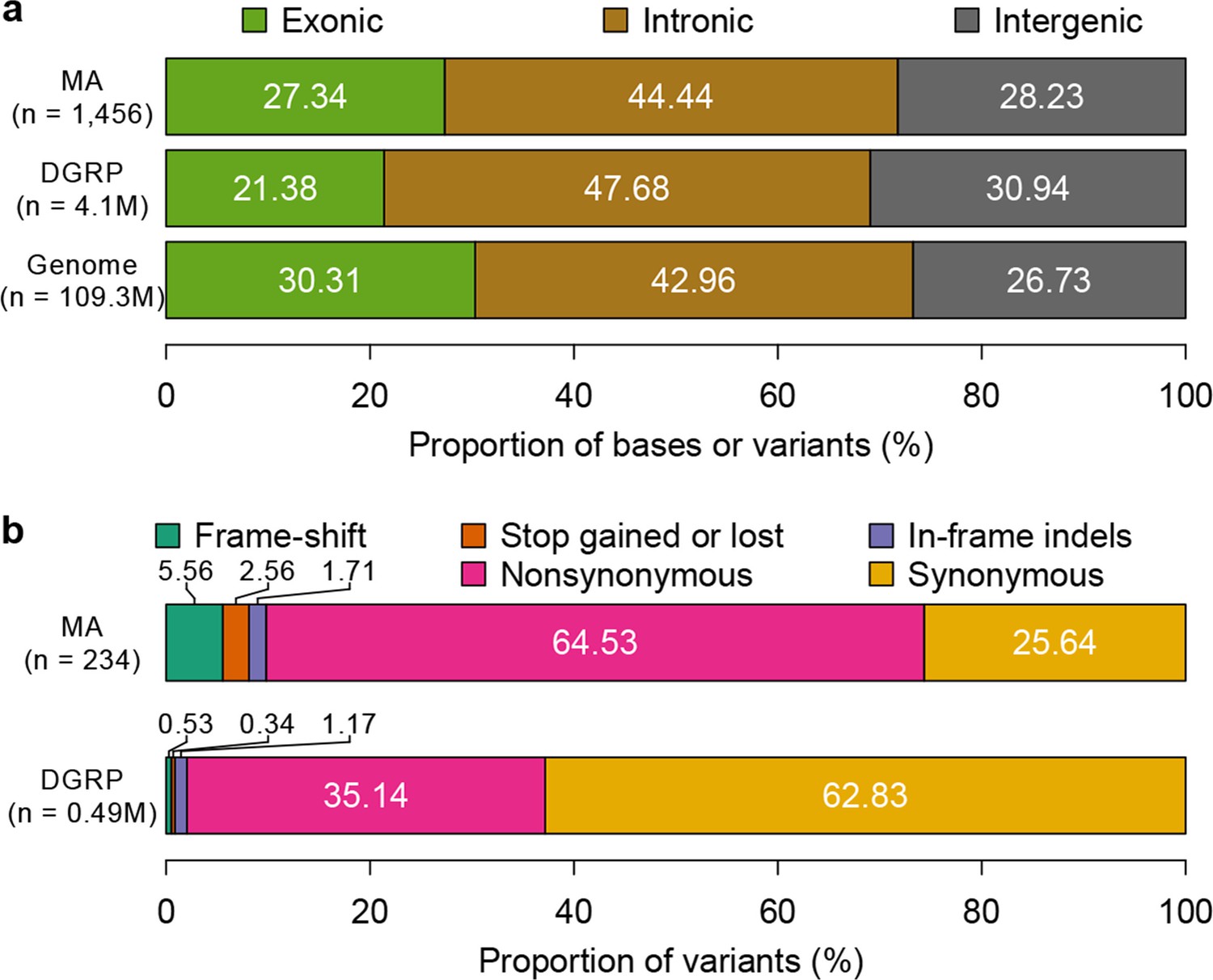
Mutation accumulation lines accumulate deleterious mutations.
Annotation of genomic bases, standing variation, and mutations in MA lines according to their (a) genomic locations and (b) functional impact on protein sequence.
Figure 6
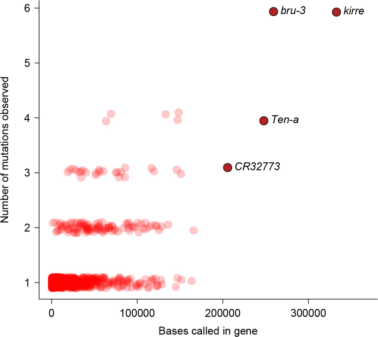
Relationship between number of mutations and gene length.
Number of mutations detected in MA lines for each gene is plotted against the total number of bases covered for mutations.
Figure 7

Inference of effective population size and mutation rate.
Expected and observed distributions of mutant allele frequency on autosomes (a) and the X chromosome (b). The expected distribution was generated based on estimates of effective population size (). Mutation rate estimates of autosomes and X chromosomes are compared for different types of mutations (c) and for different lines (d). In (d), the Pearson’s correlation coefficient (r) is calculated with (orange line) or without (green line) MA19 (orange circle).
Figure 8
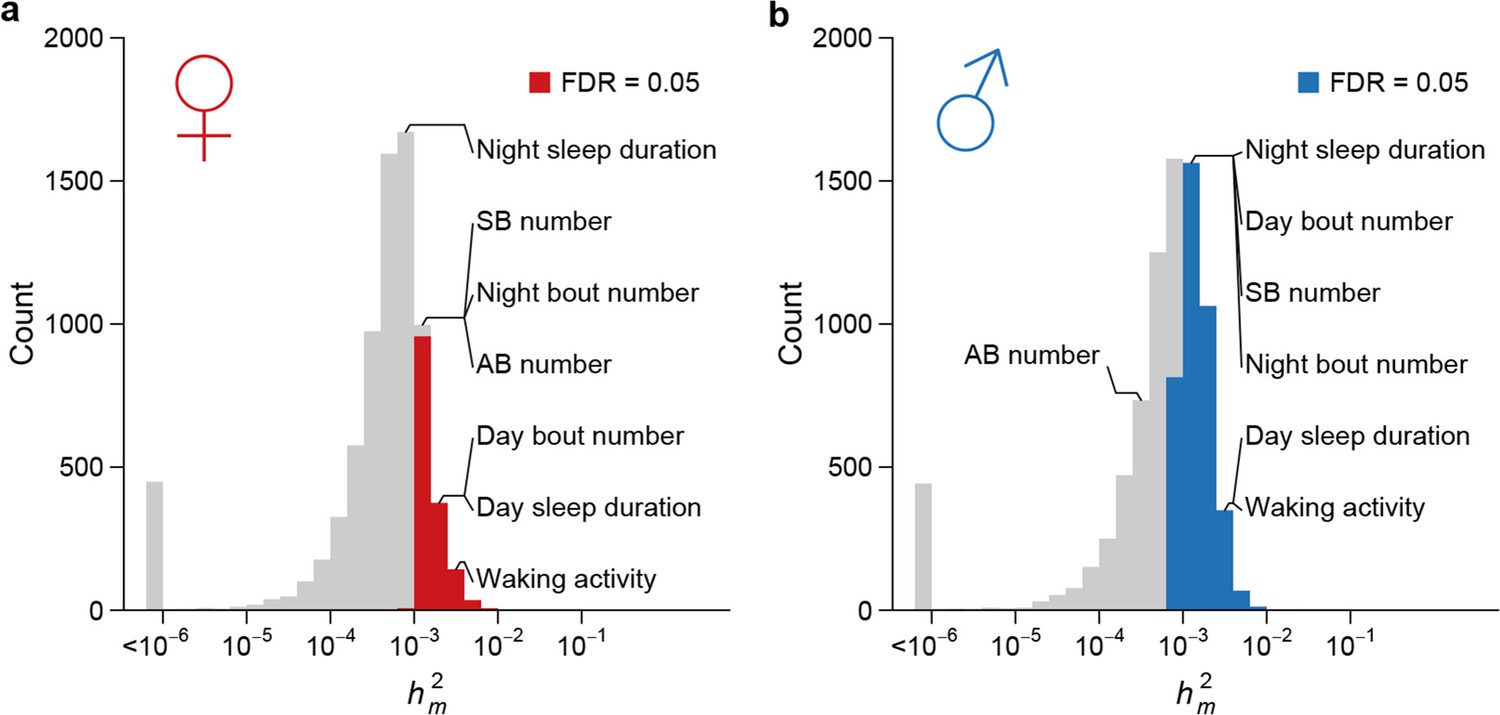
High rate of mutational variance.
Histogram of mutational heritability () for females (a) and males (b) are plotted on the log scale. The placements of organismal traits in the bins are indicated by lines connecting the bars and the trait names. AB = abdominal bristle and SB = sternopleural bristle.
Figure 9
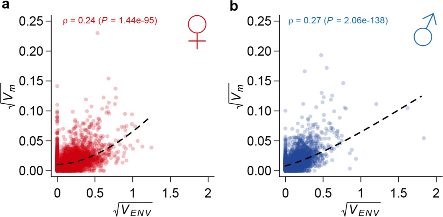
Correlation between mutational variance and environmental plasticity.
Mutational variance () is plotted against variance due to environmental plasticity () for females (a) and males (b). The dashed line is a LOESS fit to the data. Spearman’s correlation (ρ) and the P value of a test for its significance are also indicated.
Figure 10
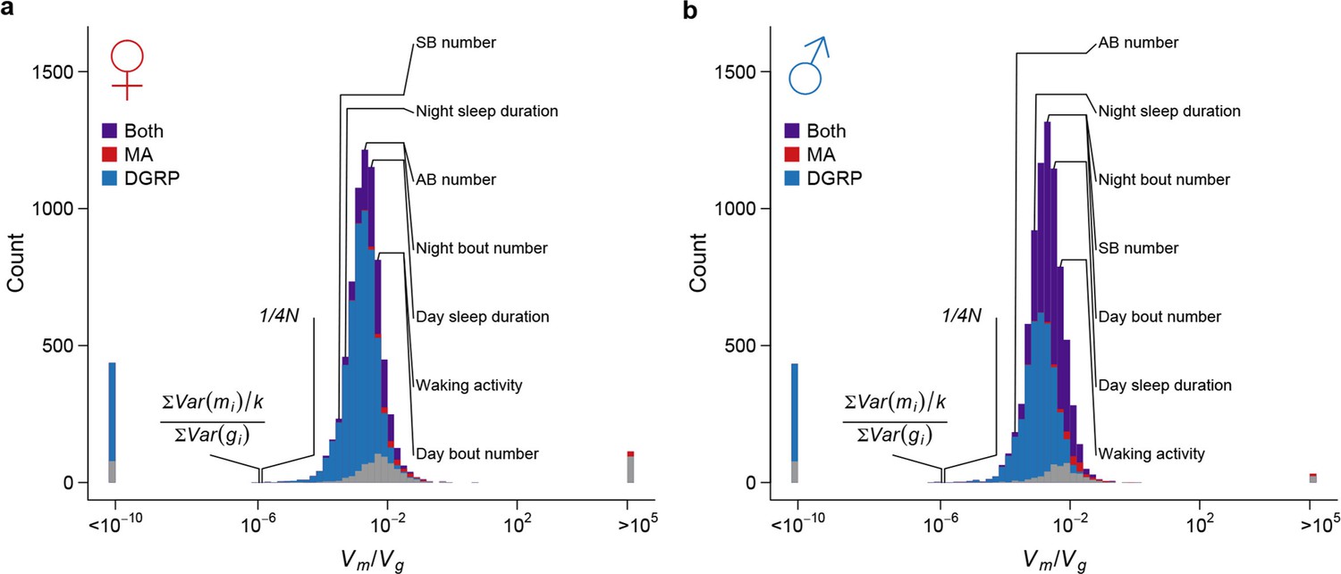
Strong apparent stabilizing selection of quantitative trait variation.
Distributions of in females (a) and males (b) are plotted on the log scale. The blue, red, and purple bars indicate genes with significant (FDR = 0.05) among-line variance in DGRP only, MA lines only, and both DGRP and MA lines respectively. Placements of organismal traits are indicated by lines connecting the bars and the trait names. AB = abdominal bristles and SB = sternopleural bristles. Neutral expectations and are also indicated.
Figure 11
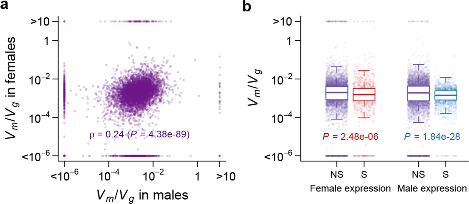
Strength of apparent stabilizing selection in females and males.
(a) for gene expression in females are plotted against that in males. (b) Boxplots of for sex-specific (S) and non-specific (NS) genes. Within each sex, for sex-specific and non-specific genes are compared using Wilcoxon’s rank sum test.
Figure 12
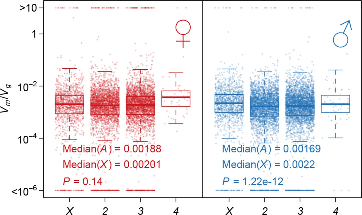
Strength of apparent stabilizing selection on autosomes and X chromosome.
Boxplots of are plotted for each chromosome in females and males. Wilcoxon’s rank sum test is used to compare on autosomes (A) and on X chromosome (X).
Figure 13
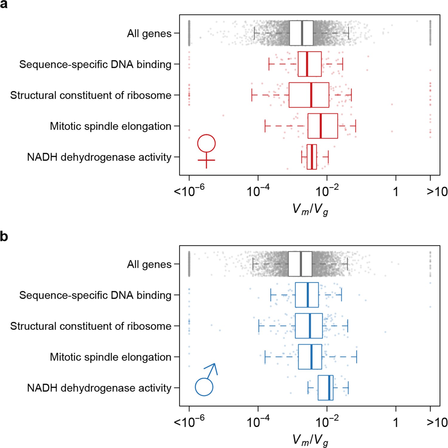
Strength of apparent stabilizing selection differs for genes in different functional categories.
Boxplots of for genes in selected Gene Ontology (GO) categories as compared to all genes.
Figure 14
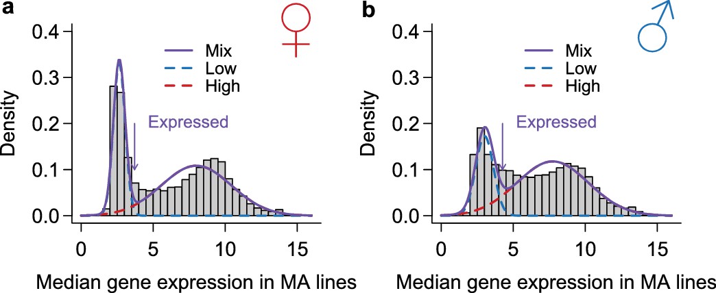
Classification of genes as expressed or not expressed in each sex.
Within each sex (females in a, males in b), the distribution of median expression for each gene across the MA lines is subject to a mixture model analysis with two normal components. The mean and variance of each component distribution is estimated using the mixtools package in R. A gene is called expressed if its posterior probability of belonging to the normal distribution with the larger mean is higher than 2/3. The histograms show the observed distribution and the estimated normal distributions and their mixture.
Additional files
-
Supplementary file 1
Supplemental tables.
(A) Summary of DNA sequencing for MA lines. (B) List of detected mutations. (C) GO enrichment analysis of mutations. (D) Variance components of organismal traits among MA and DGRP lines. (E) Variance components of gene expression traits among MA and DGRP lines. (F) Comparison of mutational variance for genes within GO categories to that of genes outside the GO categories. (G) Comparison of apparent stabilizing selection for genes within within GO categories to that of genes outside the GO categories.
- https://doi.org/10.7554/eLife.14625.017
Download links
A two-part list of links to download the article, or parts of the article, in various formats.
Downloads (link to download the article as PDF)
Open citations (links to open the citations from this article in various online reference manager services)
Cite this article (links to download the citations from this article in formats compatible with various reference manager tools)
Spontaneous mutations and the origin and maintenance of quantitative genetic variation
eLife 5:e14625.
https://doi.org/10.7554/eLife.14625


