Long-range population dynamics of anatomically defined neocortical networks
- University of Zurich, Switzerland
- University of Zurich, ETH Zurich, Switzerland
Figures
Figure 1 with 2 supplements
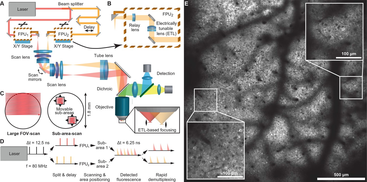
Multi-area two-photon microscope for flexible simultaneous imaging of sub-areas within a large field-of-view.
(A) Schematic of multi-area two-photon microscope. Light from a Ti:sapphire laser is split into two beams and one beam sent to a delay line. Each beam then enters a focal plane unit (FPU), which allows axial focusing with an electrically tunable lens (ETL). Both beams are scanned in parallel by a pair of galvo mirrors. (B) Schematic of FPU. (C) Imaging modes include scanning of a single large FOV (with one beam switched off) and parallel scanning of two sub-areas. (D) Principle of spatiotemporal multiplexing: The detected fluorescence photons can be attributed to the correct area of origin by rapid demultiplexing synchronized to the laser pulse train. (E) Example two-photon image (1.7 mm FOV) at 160–180 µm depth in a YCX2.60-expressing transgenic mouse in L2/3.
Figure 1—figure supplement 1
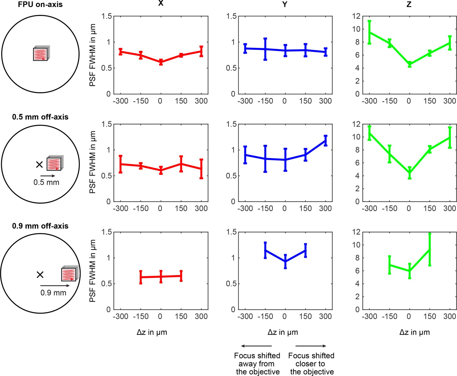
Variation of the point-spread function over field-of-view position and ETL tuning range.
The point-spread function (PSF) was measured using 200 nm beads (Fluoresbrite Plain YG Microspheres, Polysciences Inc) at 840 nm excitation. Off-axis positions were accessed by translating a focal plane unit (FPU) to a position corresponding to a sample-offset of 500 μm and 900 μm. Full-width-half-maxima (FWHM) of the PSF are shown for the x-, y-, and z-direction. The PSFs exhibit residual astigmatism and degrade when the focus is moved away from the nominal working distance (∆z = 0) and the on-axis position. Due to vignetting, the ETL tuning range is limited at 900 μm off-axis. n = 5 beads, error bars: 95% confidence interval.
Figure 1—figure supplement 2
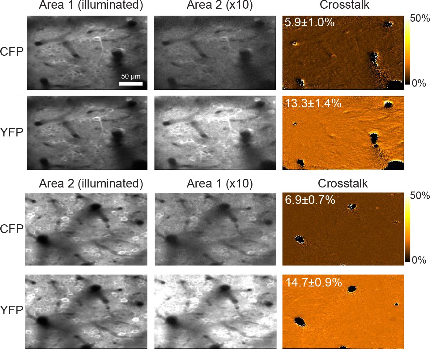
Crosstalk between both sub-areas observed in vivo.
Neurons expressing YC-Nano140 were imaged with a single beam exciting fluorescence either in sub-area 1 or 2 (Average of n = 49 frames with motion correction). The detected signal in the non-illuminated sub-area is due to crosstalk caused by the exponential fluorescence decay (shown amplified by a factor of 10 for better visibility). The crosstalk can be quantified by the ratio of both images after background subtraction (the background was estimated from a ROI placed in the dark blood vessels). The percent crosstalk estimates are averages over 10000 pixels excluding blood vessels with standard deviation. As CFP is quenched by YFP in the Förster resonance energy transfer (FRET) interaction between both fluorophores, the lifetime of the CFP emission is shortened, which leads to a lower crosstalk.
Figure 2 with 1 supplement
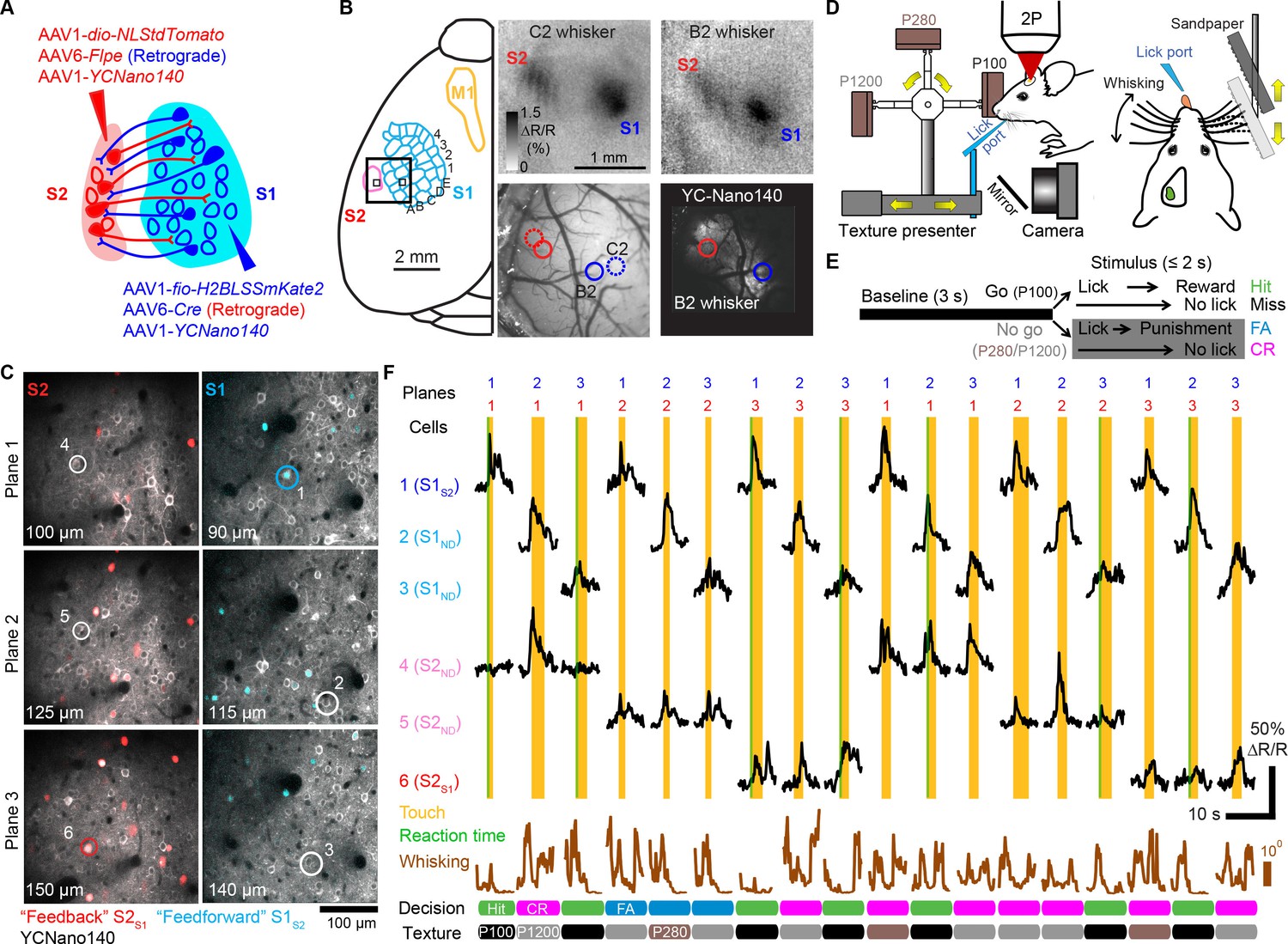
Simultaneous calcium imaging of identified feedforward and feedback neurons in S1 and S2 of mouse neocortex during behavior.
(A) Viral injection scheme for simultaneous labeling of feedforward and feedback neurons and YC-Nano140 expression. (B) Functional mapping of S1 and S2 through optical intrinsic signal imaging. Intrinsic signals evoked by stimulation of the C2 whisker (top left) and the B2 whisker (top right). In addition to localized intrinsic signals in S1 barrel columns, additional activation spots are visible in S2. Identified barrel columns (circles) are overlaid over blood vessel (bottom left) and YC-Nano140 expression (bottom right) images. (C) In vivo 2-photon images of LSSmKate2-positive S1S2 neurons (blue), tdTomato-positive S2S1 neurons (red) with non-co-labeled YC-Nano140-expressing neurons (grey) in S1 (S1ND) and S2 (S2ND). (D) Behavior setup for texture discrimination task. (E) Trial structure for go/no-go texture discrimination task. (F) Example calcium transients for individual neurons in [C] measured episodically during texture discrimination task along with periods of whisker-to-texture touch (orange area), whisking amplitude (brown trace), and reaction time on Hit trials (green area). For each trial the selected plane in each sub-area is indicated on top, illustrating the combinatorial plane hopping.
-
Figure 2—source data 1
Optimized low tensor rank across animals.
Table of optimum column size of each factor matrices related to neurons (N’ + N’offset), time points (T’), and trial conditions (C’) determined after cross-validation and cost function procedures for each animal used for denoising. Total possible column sizes are also indicated along with number of active neurons.
- https://doi.org/10.7554/eLife.14679.008
Figure 2—figure supplement 1
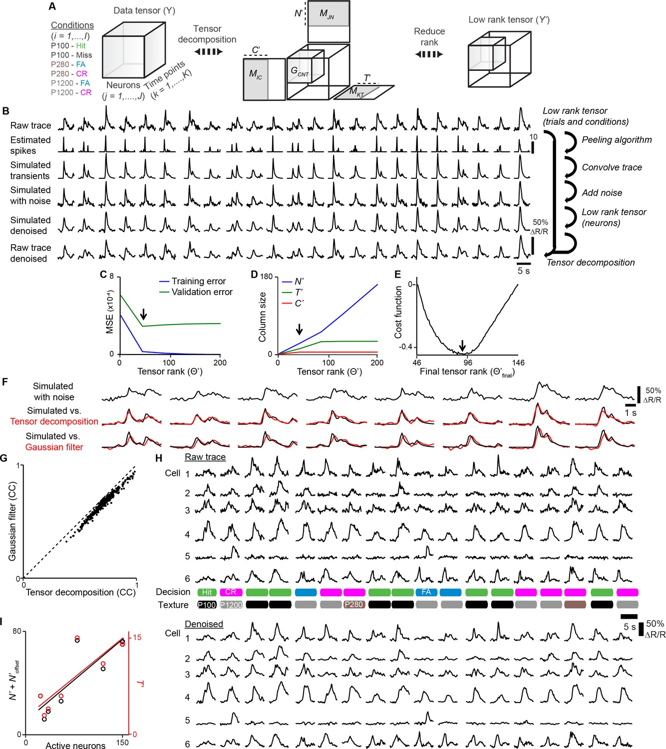
Denoising with tensor decomposition.
(A) Calcium responses from one animal across multiple sessions are organized into a data tensor. The tensor is decomposed and a low-rank tensor representing denoised calcium responses is generated. (B) Denoising procedure: A low-rank tensor for trials and conditions was determined by cross-validation methods. A low-rank tensor for neurons was determined by convolving estimated spike trains from experiment data to generate simulated calcium traces. Noise is added to simulate calcium traces and tensor decomposition is performed to determine an optimum low-rank tensor by comparing simulated vs. simulated denoised traces. Once an optimum low rank tensor is determined for all dimensions, tensor decomposition is applied to raw traces. (C) Low tensor rank (arrow) computed by cross-validation of training set. (D) Contribution of each dimension to low tensor rank in [C]. (E) Final low tensor rank offset (arrow) computed by cost function of simulated vs. simulated denoised traces. (F) Comparison of simulated traces denoised with tensor decomposition vs. Gaussian filter. (G) Denoised fits from Gaussian filter vs. tensor decomposition for single neurons from simulated data. (H) Example of experimental data before and after denoising. (I) Optimum T’ or N’ + N’offset vs. active neurons for each animal.
Figure 3 with 1 supplement
Feedback neurons in S2 exhibit behavior-related responses.
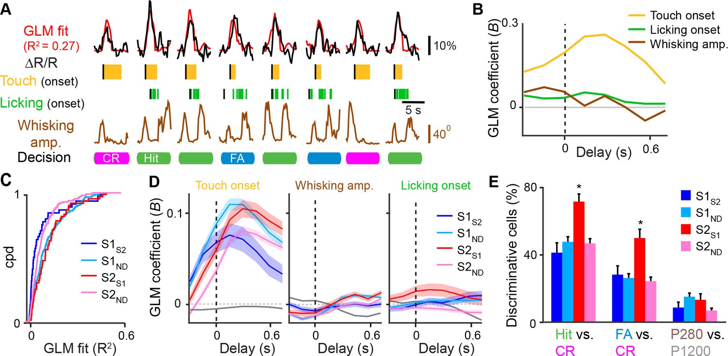
(A) General linear model (GLM) of behavior-related responses. Example of GLM fit for one neuron of calcium responses against touch, licking, and whisking as behavior events. Single-trial calcium responses are plotted along with model fit as well as touch periods with onset indicated, individual licks with onset indicated, whisking envelope amplitude, and decision. (B) GLM coefficients (B) for example neuron shown in [A] for regressors for touch onset, whisking envelope amplitude, and licking onset across different delays. Delays are aligned to the onset of each behavioral event. (C) Cumulative probability distribution (cpd) of overall GLM fit across cell types. (D) GLM coefficients for different cell types for regressors for touch onset (left), whisking envelope amplitude (middle), and licking onset (right) across different delays. Grey line indicates average GLM coefficient for neurons with non-significant coefficients at that time point. (E) Fraction of active neurons able to discriminate Hit vs. CR, FA vs. CR, and P280 vs. P1200 trials above chance determined by single-cell ROC analysis. (shaded area: s.e.m. error bars: s.d. from bootstrap test; n = 44 S1S2, 161 S1ND, 59 S2S1, 198 S2ND neurons).
Figure 3—figure supplement 1
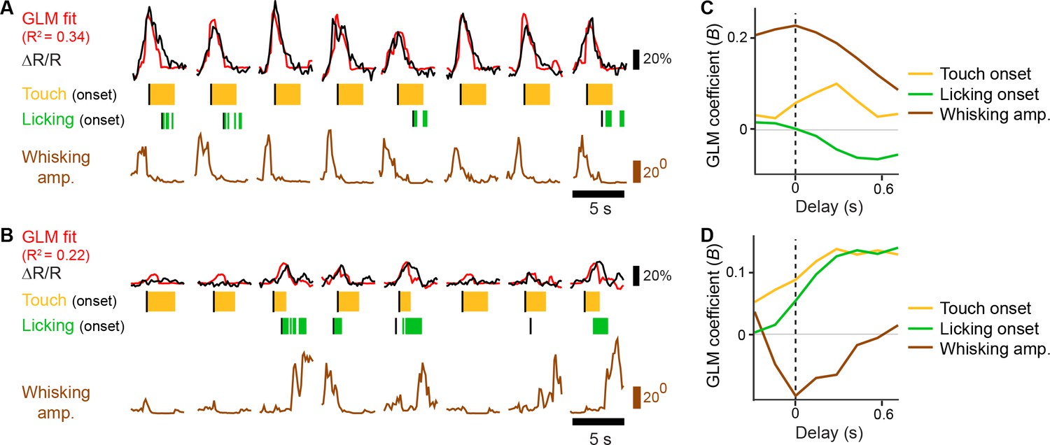
General linear model of whisking- and licking-related calcium responses.
(A–B) Example of GLM fit for neurons showing prominent whisking [A] and licking [B] related calcium responses against touch, licking, and whisking behavior events. Single-trial calcium responses are plotted along with model fit as well as touch periods with onset indicated, individual licks with onset indicated, and whisking envelope amplitude. (C–D), GLM coefficients (B) for neurons in [A] and [B], respectively, for regressors for touch onset, whisking envelope amplitude, and licking onset across different delays. Delays are aligned to the onset of each behavioral event.
Figure 4
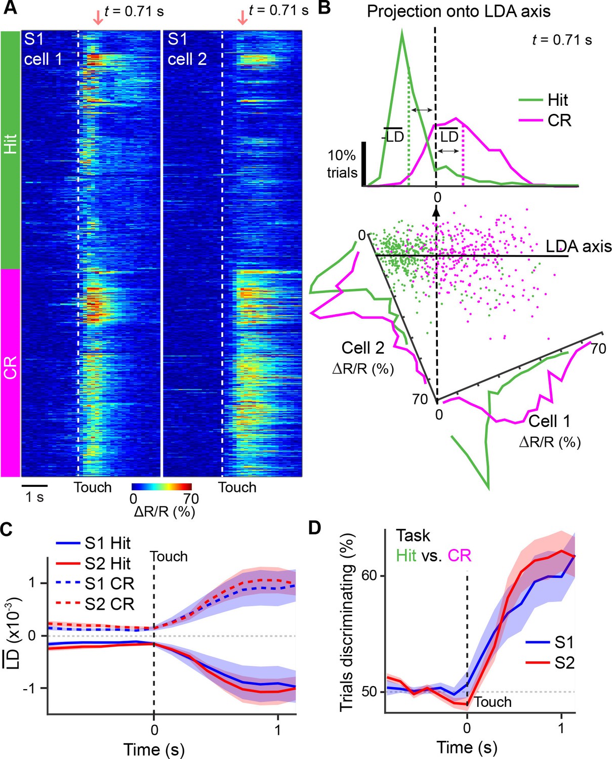
Illustration of extracting population response time courses by linear discriminant analysis.
(A) While LDA is performed on multiple simultaneously imaged neurons, for demonstration purposes, here calcium transients of two simultaneously imaged neurons within an imaging plane are plotted and sorted according to Hit and CR trials. Dotted line indicates whisker-touch onset. (B) Example linear discriminant analysis performed on the two neurons in [A]. Bottom panel shows scatter plot of trial-by-trial responses for each neuron at the indicated time point (red region in [A]) rotated along the LD axis for Hit vs. CR trials. Top panel shows distribution of trials for population activity projected along the LD axis along with mean LD response. (C) Average S1 or S2 population responses after LDA in Hit and CR trials across the first second prior to and following whisker-touch onset. (D), ROC analysis of S1 or S2 population responses shown in [C] for Hit vs. CR trials under task conditions demonstrating the performance of the LDA. Dotted line indicates touch onset. (shaded area: s.e.m.; n = 21 S1 planes, 21 S2 planes).
Figure 5 with 2 supplements
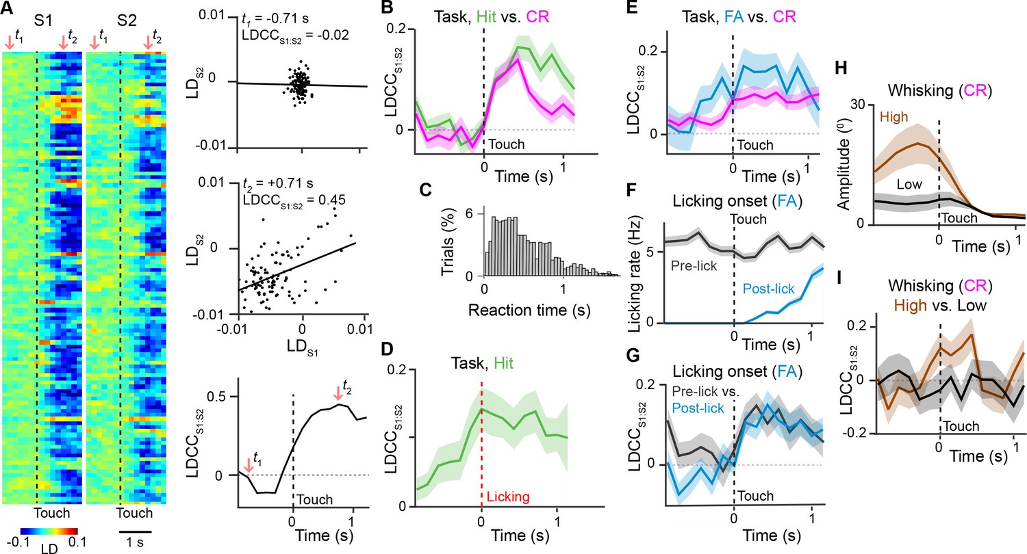
Motor behavior is associated with coordinated population activity across S1 and S2.
(A) Analysis of coordinated activity across S1 and S2. Left panel shows example of single-trial population responses for Hit trials projected along Hit vs. CR axis for simultaneously imaged S1 (LDS1) and S2 (LDS2) of S2 sub-areas. Upper right panels shows trial-by-trial correlations (LDCCS1:S2) between LDS1 andLDS2 atindicated time points. Bottom right panel shows calculated LDCCS1:S2 across the trial period. (B) LDCC S1:S2 for Hit vs. CR trials. (C) Normalized histogram of reaction times across Hit trials. (D) LDCC S1:S2 for Hit trials along Hit vs. CR axis aligned to licking onset. (E) LDCC S1:S2 for FA vs. CR trials. (F) Licking rate for FA trials in which licking onset precedes (pre-wo) and follows (post-wo) whisker-touch onset. (G) LDCC S1:S2 for pre-wo vs. post-wo FA trials. (H) High vs. low whisking amplitude CR trials. (I) LDCC S1:S2 for high vs. low whisking amplitude CR trials. All time course data are aligned to whisker-touch onset (black dotted line, x-axis) except for [D] which is aligned to licking onset (red dotted line). shaded area: s.e.m.; (C,D,E,G,I) n = 63 pairs of S1 and S2 planes in 7 animals; (C) n = 7120 trials (F) n = 1120 trials (H) n = 7 animals, 6960 trials.
Figure 5—figure supplement 1
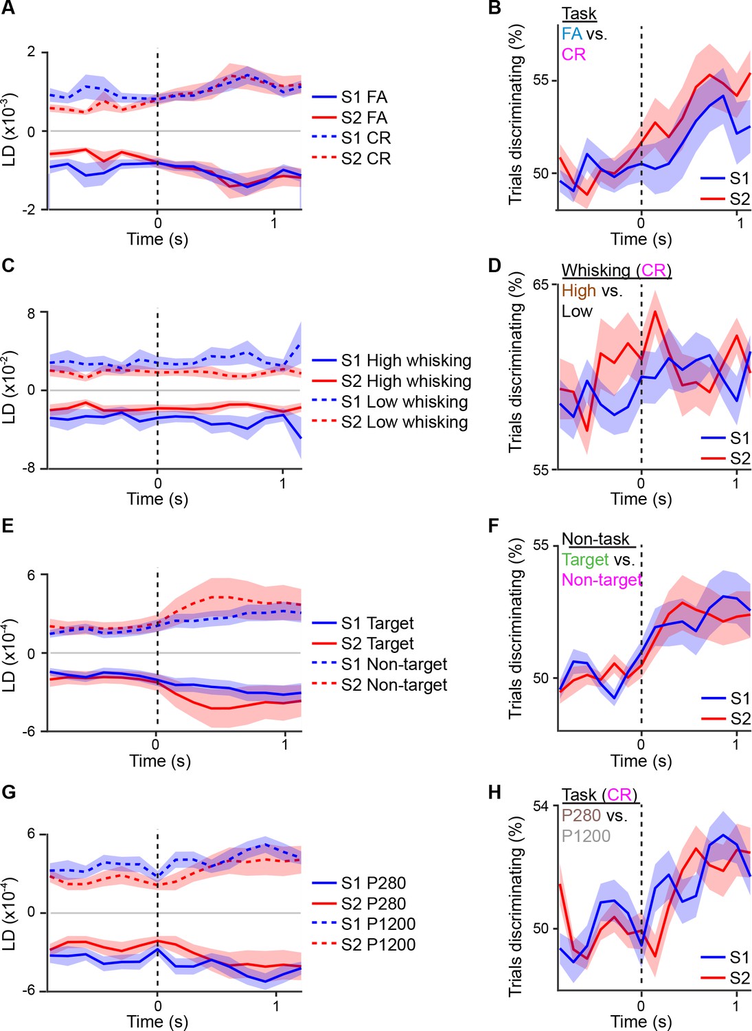
Linear discriminant analysis across different sensory or behavior axes.
Average S1 or S2 population responses across the first second prior to and following whisker touch onset for: (A) FA vs. CR trials; (C) high- vs. low-amplitude whisking CR trials; (E) target vs. non-target textures under non-task conditions; G, P280 vs. P1200 textures for CR trials. ROC analysis of S1 or S2 population response for: (B) FA vs. CR trials; (D) high- vs. low-amplitude whisking CR trials; (F) target vs. non-target textures under non-task conditions; (H) P280 vs. P1200 textures for CR trials. Dotted line indicates touch onset. (shaded area: s.e.m.; n = 21 S1 planes, 21 S2 planes)
Figure 5—figure supplement 2
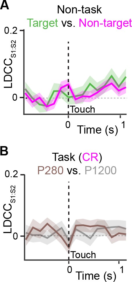
Coordinated actitvity across S1 and S2 is not stimulus-specific.
(A) LDCCS1:S2 for target vs. non-target textures under non-task condition trials. (B) LDCCS1:S2 for P280 vs. P1200 textures for CR trials. We observed no increased or different LDCCS1:S2 between target and non-target textures under non-task conditions when animals received sensory stimulation but neither whisked nor licked. We also observed no increase or difference in LDCCS1:S2 when analyzing population responses for P280 vs. P1200 textures on CR trials under task conditions. All time course data are aligned to whisker-touch onset (black dotted line, x-axis). shaded area: s.e.m.; n = 63 pairs of S1 and S2 planes in 7 animals.
Figure 6 with 3 supplements

Projection neurons contribute to coordinated S1 and S2 activity.
(A) The contribution of specific cell types to coordinated activity across S1 and S2 is measured by trial-shuffling responses for those cell types prior to calculating the LDCCS1:S2. The resulting LDCCS1:S2 from the shuffled condition is then subtracted by the LDCCS1:S2 from the control condition to obtain ∆LDCCS1:S2 (see also Figure 6—figure supplement 1). (B), ∆LDCCS1:S2 for Hit trials along the Hit vs. CR axis after aligning to licking onset. (C) ∆LDCCS1:S2 for high-amplitude whisking CR trials along the high vs. low whisking amplitude CR trial axis. (D) ∆LDCCS1:S2 for FA trials, in which licking onset precedes whisker-touch onset along the FA vs. CR axis. (E) ∆LDCCS1:S2 for FA trials, in which licking onset follows whisker-touch onset along the FA vs. CR axis. (F) ∆LDCCS1:S2 for CR trials along the FA vs. CR axis. All time course data are aligned to whisker-touch onset (dotted line, x-axis) except for [B] which is aligned to licking onset (red dotted line). (shaded area: s.e.m.; n = 21 S1 planes, 21 S2 planes, 63 pairs of S1 and S2 planes in 7 animals).
Figure 6—figure supplement 1
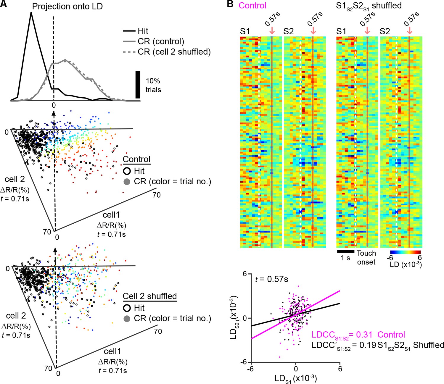
Measuring the contribution of specific cell types to coordinated population activity.
(A), An example of population response after trial shuffling. Trial responses of neuronal subpopulations were shuffled in order to determine their contribution to the population response. For the two example neurons also shown in [Figure 4A,B], the contribution of ’cell 2‘ on the population response for Hit trials was examined by shuffling the order of trial responses for’ cell 2‘. A scatter plot of the trial-by-trial responses of ’cell 1‘ vs. ’cell 2‘ is shown before (middle) and after (bottom) shuffling. The corresponding trials in control and shuffled conditions are indicated by color. The population responses under shuffled conditions were projected onto the LD axis for Hit vs. CR trials determined under control conditions (top). (B) Example analysis of coordinated activity across S1 and S2 after trial shuffling. Single-trial population responses for CR trials projected along the FA vs. CR axis for simultaneously imaged S1 (LDS1) and S2 (LDS2) sub-areas are shown under control conditions (top left) and after shuffling trials of S1S2 and S2S1 neurons (top right). Bottom panel shows trial-by-trial correlations (LDCCS1:S2) between LDS1 and LDS2 at indicated time point for control and shuffled conditions. See [Figure 6A,B] for subsequent analysis of the same sub-areas to measure △LDCCS1:S2 across the trial period.
Figure 6—figure supplement 2
Projection of shuffled trials does not alter average population response.
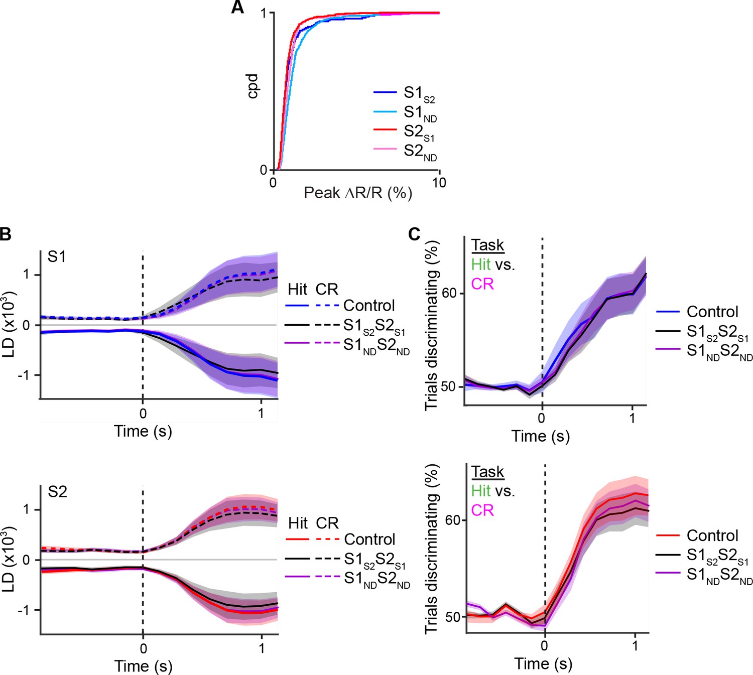
(A) Cumulative distribution of average peak calcium responses for each cell type. (B) Average S1 (top) or S2 (bottom) population responses projected along the Hit vs. CR axis across the first second prior to and following whisker-touch onset in data in which no trials are shuffled (control), trials of S1S2 and S2S1 neurons are shuffled (S1S2S2S1), and S1ND and S2ND neurons are shuffled (S1NDS2ND). (C) ROC analysis of S1 (top) or S2 (bottom) population responses, in which no trials are shuffled (control), trials of S1S2 and S2S1 neurons are shuffled (S1S2S2S1), and S1ND and S2ND neurons are shuffled (S1NDS2ND) vectors for Hit vs. CR trials under task conditions. Dotted line indicates touch onset. (shaded area: s.e.m.; n = 21 S1 planes, 21 S2 planes).
Figure 6—figure supplement 3
Contribution of S1S2 and S2S1 neurons to Hit and CR trials relative to whisker-touch onset.
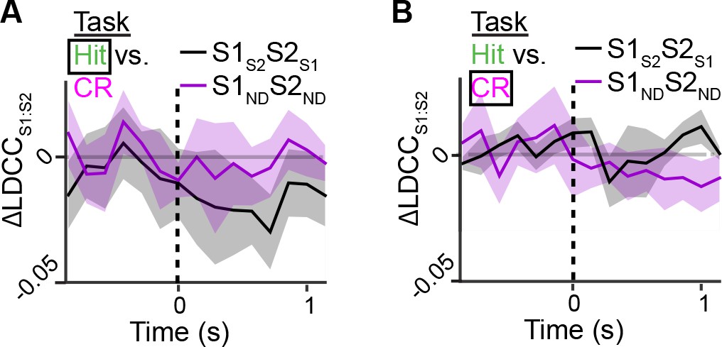
(A) Contribution of S1S2 and S2S1 neurons or S1ND and S2ND neurons to coordinated S1 and S2 activity for Hit trials along the Hit vs. CR axis after aligning to whisker-touch onset (dotted line). (B) Contribution of S1S2 and S2S1 neurons or S1ND and S2ND neurons to coordinated S1 and S2 activity for Hit trials along the Hit vs. CR axis after aligning to whisker-touch onset. (shaded area: s.e.m.; n = 63 pairs of S1 and S2 planes in 7 animals).
Figure 7
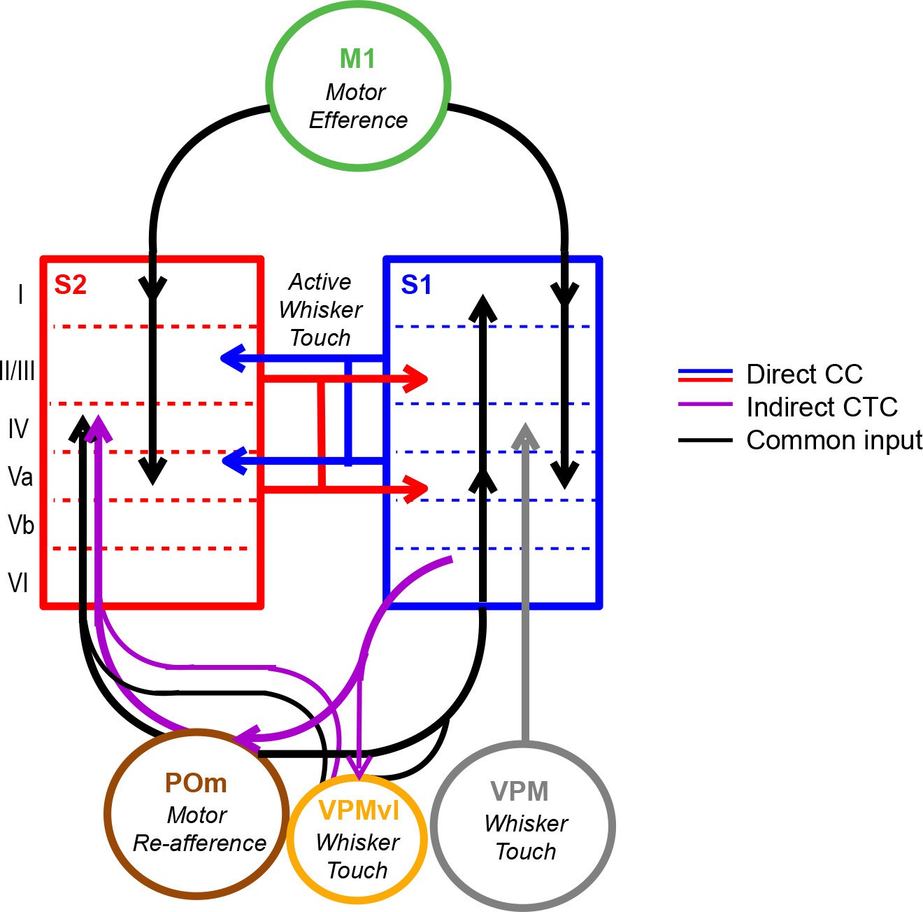
Model of coordinated activity across S1 and S2.
Our results identify coordinated activity patterns across S1 and S2 that are related to motor behaviors, which could arise from common input from M1 or POm or indirect cortico-thalamocortical (CTC) pathways through POm. S1S2 and S2S1 neurons especially participate in inter-areal coordination when motor behavior is paired with sensory stimuli suggesting that such cortico-cortical (CC) interactions specifically reflect the exchange of sensory information during active sensation.
Videos
Video 1
In vivo z-stack of YC-Nano140 expressing neurons.
Single area images from the multi-area two-photon microscope of L2/3 neurons were taken from 70-210 µm below the pial surface at 1 µm z-step resolution. Sub-area excitation beam was delivered through the ETL, positioned either on-axis (left) or 900 µm off-axis (right), and focusing was achieved through translation of the objective by the z-stage.
Video 2
Simultaneous calcium imaging across S1 and S2.
Single trial video of calcium responses during texture discrimination acquired at 7 Hz with the multi-area two-photon microscope (1x playback speed). YFP (green) and CFP (blue) fluorescence from YC-Nano140 are shown and overlaid with calculated ∆R/R (red).
Tables
Table 1
Axes used for linear discriminant analysis. Summary of trial conditions compared and used for linear discriminant analysis. For each axes, noted are potential differences in texture, licking, and whisking parameters between trial conditions as well as the utility in comparing such trial conditions for isolating sensory or behavior responses.
| Axes for LDA | Texture | Licking | Whisking | Utility in analysis |
|---|---|---|---|---|
| Hit vs. CR | Different | Different (Hit) | Same | Cannot isolate sensory, decision, or action-related responses |
| FA vs. CR | Same | Different (FA) | Same | Isolate decision and action-related responses |
| Pre- vs. post-touch licking (FA trials) | Same | Different | Same | Isolate licking-related responses |
| High vs. Low Whisking (CR trials) | Same | None | Different | Isolate whisking-related responses |
| P280 vs. P1200 (CR trials) | Different | None | Same | Isolate sensory-related responses |
| Target vs. Non-target (Non-task) | Different | None | None | Isolate sensory-related responses |
Download links
A two-part list of links to download the article, or parts of the article, in various formats.
Downloads (link to download the article as PDF)
Open citations (links to open the citations from this article in various online reference manager services)
Cite this article (links to download the citations from this article in formats compatible with various reference manager tools)
Long-range population dynamics of anatomically defined neocortical networks
eLife 5:e14679.
https://doi.org/10.7554/eLife.14679


