A Bayesian model of context-sensitive value attribution
- University College London, United Kingdom
- King's College London, United Kingdom
- Sismanoglio General Hospital, Greece
- Max Planck UCL Centre for Computational Psychiatry and Ageing Research, United Kingdom
Figures
Figure 1
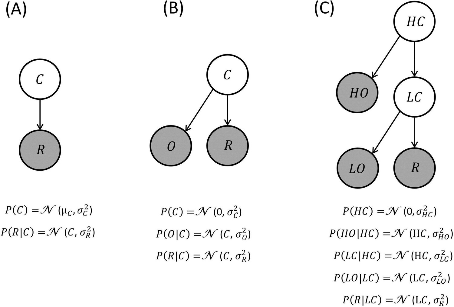
Generative models of reward: these generative models are depicted as directed acyclic graphs or Bayesian networks.
Circles represent random variables (shaded and white circles refer to observed and non-observed variables respectively). An arrow denotes a conditional dependence – in which one random variable supplies a sufficient statistic of the probability distribution of its children. In BCV, contextual variables generate the sufficient statistics (expectation and variance) of a Gaussian observable variable corresponding to reward. In these examples, the contextual variables generate first-order sufficient statistics of their descendants (e.g., the mean of Gaussian distributions) as in parametric or empirical Bayesian models. Alternatively, the contextual variables could determine the variance of Gaussian random variables; in which case this would be a hierarchical Gaussian filter. Inverting this model, given observations, furnishes posterior beliefs over the context variables. This inference determines incentive value which is conceived as precision-weighted prediction error. (A) Generative model where a contextual variable C reflects a prior belief over the reward mean. (B) Generative model where a contextual variable C generates a prior expectancy of zero over the reward mean, and a noisy observation O of the context is provided. (C) Generative model where context is organized hierarchically and comprises a high level (HC; e.g., a neighbourhood) and a low level (LC; e.g., a restaurant), both associated with noisy observations (HO and LO respectively).
Figure 2
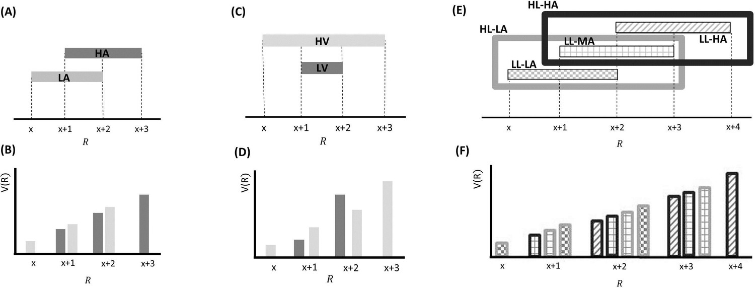
Effects predicted by BCV on the incentive value (V(R)) as a function of reward (R) and contexts associated with specific distributions of rewards presented sequentially over trials arranged in blocks.
(A) Example with a single hierarchical level where two contexts have different average reward. In blocks associated with a low-average context (LA; in lighter grey), the possible rewards are x, x+1 and x+2; in blocks associated with a high-average context (HA; in darker grey), the possible rewards are x+1, x+2 and x+3. (B) BCV prediction of the incentive value attributed to rewards depending on these contexts. Larger values are predicted in the LA compared to the HA for amounts common to both contexts. (C) Effects predicted by BCV dependent on contexts with different reward variance. In blocks associated with a high-variance context (HV; in lighter grey), the possible rewards are x, x+1 x+2 and x+3; in blocks associated with a low-variance context (LV; in grey), the possible rewards are x+1 and x+2. (D) BCV prediction of the incentive value attributed to rewards depending on these contexts. Considering rewards common to both contexts, BCV predicts a higher incentive value for x+1 in the high-variance context and for x+2 in the low-variance context. (E) Example with two hierarchical levels (low-level (LL) contexts, represented by patterns of bars, and high-level (HL) contexts, represented by frames). Blocks associated with HL contexts comprise several sub-blocks associated with LL contexts having specific average reward. In the HL context with low-value (HL-LA; light frame), a LL context with low value (LL-LA, where rewards are x, x+1 and x+2) and a LL context with a medium value (LL-MA, where rewards are x+1, x+2 and x+3) alternate. In the HL context with high-value (HL-HA; dark frame), a LL-MA context and a LL context with high value (LL-HA, where rewards are x+2, x+3 and x+4) alternate. (F) BCV prediction of the incentive value attributed to rewards depending on these hierarchical contexts. The pattern of bars represents the LL context condition, the outline colour represents the HL context condition. BCV predicts that incentive values derive from integrating both hierarchical levels, with larger values emerging when the average reward is lower at both context levels.
Figure 3

Behavioural paradigm.
On each trial, participants were presented a monetary amount (£8 in this example) in the middle of the screen and had to choose between half of the amount for sure (pressing a left button) and a gamble (pressing a right button) associated with either the full amount or a zero outcome, each with an equal chance. The outcome was shown right after response for one second. During the intertrial interval (ITI), the possible amounts of the next trial were shown on the top of the screen in brackets. The same amounts were presented throughout blocks associated either with a low-variance (LV) context, including £6 and £8 amounts, or a high-variance (HV) context, including £4, £6, £8 and £10 amounts.
Figure 4 with 1 supplement
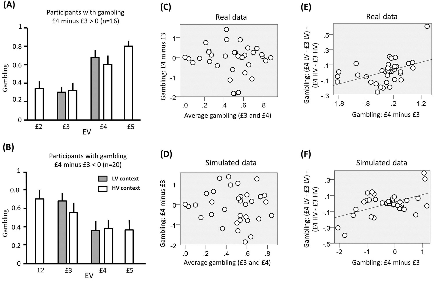
Results of experiment one (data used for the analyses reported here are provided in Source code 1).
(A) Gambling proportion for different EVs and contexts for participants who gambled more for £4 compared to £3 choices. (B) Gambling proportion for different EVs and context for participants who gambled less for £4 compared to £3 choices. (C) Relationship between average gambling proportion for £3 and £4 EV choices and gambling proportion for £4 minus £3 choices. Data showed no correlation (r(36) = -0.06, p = 0.75). (D) The same relationship is reported for data simulated with the computational model of choice behaviour and the parameters estimated from choice behaviour (r(36) = −0.03, p = 0.87). (E) Relationship between (i) the gambling proportion for £4 minus £3 choices and (ii) the interaction term reflecting the gambling proportion for £4 minus £3 choices in the low-variance context compared to the gambling proportion for £4 minus £3 choices in the high-variance context. Data showed a positive correlation (r(36) = 0.45, p = 0.005). Note that this result remains significant also using Spearman correlation, which is less affected by outliers (rho = 0.51, p = 0.002). (F) The same relationship is reported for data simulated with the computational model of choice behaviour and the parameters estimated from choice behaviour (r(36) = 0.48, p = 0.003; the plot reports an example taken from the 100 simulations).
Figure 4—figure supplement 1
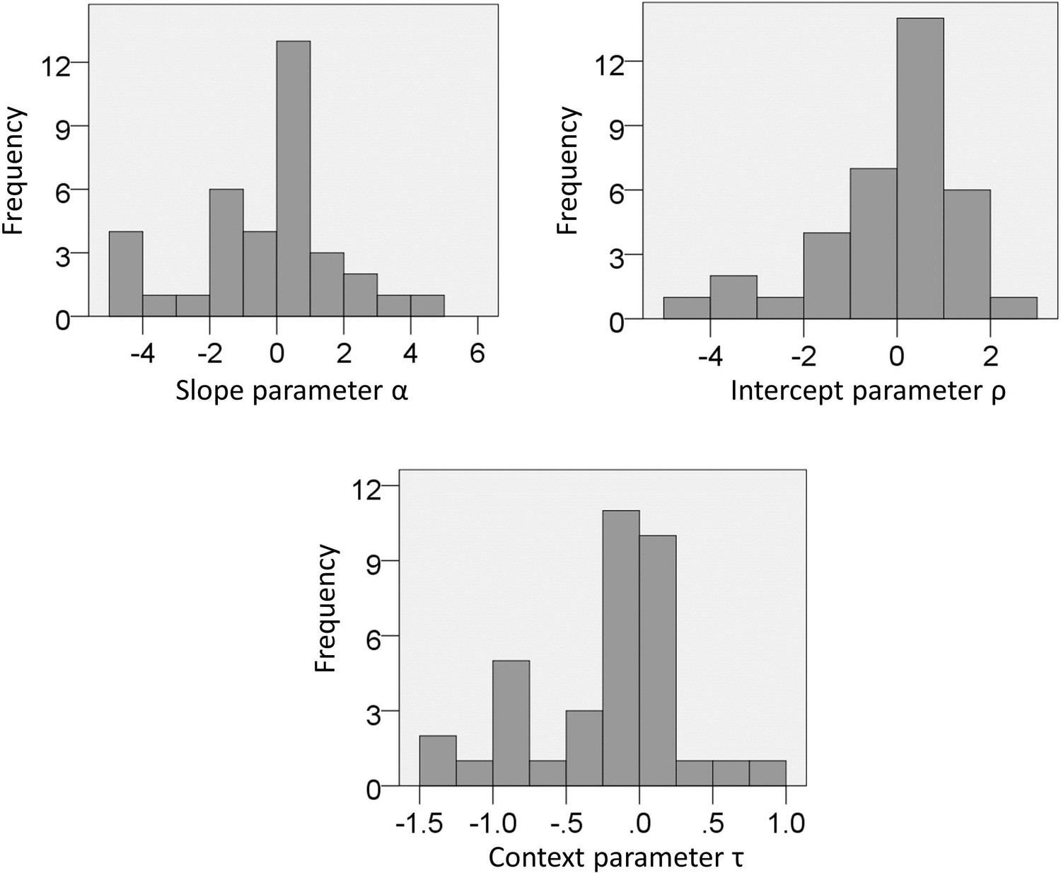
Experiment one: distribution of parameters estimated from choice data with the full model.
https://doi.org/10.7554/eLife.16127.006
Figure 5
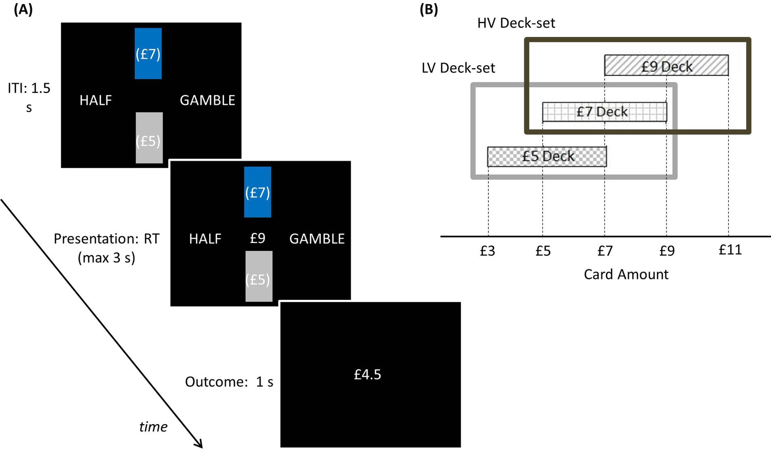
Experimental paradigm: participants played a computer-based task where, on each trial, two rectangles representing two decks of cards appeared.
(A) Each card was associated with a monetary gain, and the average monetary gain of each deck was displayed in brackets on the deck. The decks were coloured one in blue and the other in grey, indicating the selected and unselected deck respectively. Among these two decks shown on the screen, the selected deck (coloured in blue) alternated pseudo-randomly over blocks (each including 5 trials). In addition, two sets of decks alternated over longer blocks (20 trials) in a pseudo-random way. After decks were shown during an inter-trial-interval of 1.5 s, a card was pseudo-randomly drawn from the blue deck and the corresponding monetary amount was presented in the middle of the screen. Participants had to choose between half of the monetary amount for sure (pressing a left button) and a gamble between the full amount and a zero outcome (pressing a right button), each with a 50% chance. After choosing, the choice outcome appeared for one second. At the end of the experiment, one outcome was randomly selected and paid to participants. (B) Schematic of how contexts are organized in this paradigm. The selected deck alternated pseudo-randomly over blocks. In addition, two sets of decks alternated over longer blocks in a pseudo-random way. The low-value deck-set (LV Deck-set; light grey frame) comprised decks associated with £5 and £7 on average; the high-value deck-set (HV Deck-set; dark grey frame) comprised decks associated with £7 and £9 on average. The cards of the £5 deck could be associated with £3, £5 and £7; the cards of the £7 deck could be associated with £5, £7 and £9; the cards of the £9 deck could be associated with £7, £9 and £11.
Figure 6
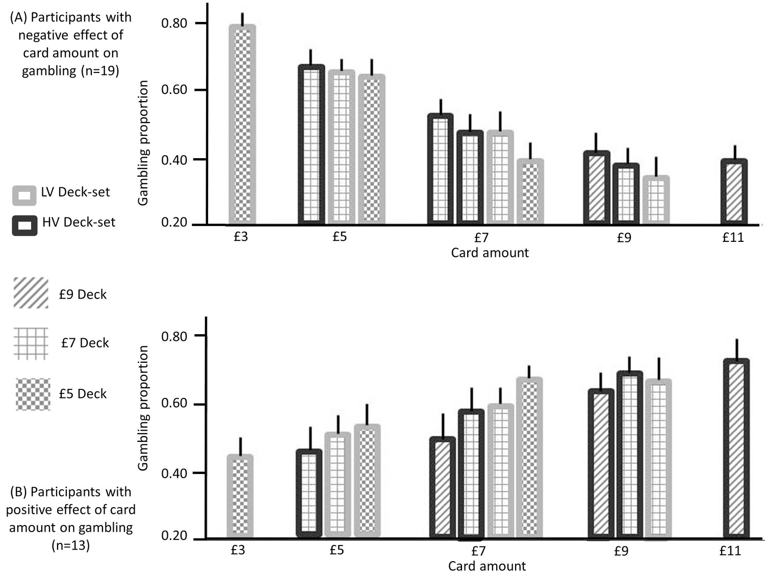
Gambling proportion for different card amounts and different context conditions (data used for this figure are provided in Source code 2), separately for (A) participants showing a negative effect of card monetary amount (i.e., the slope of the logistic regression model with card amount as a predictor) on gambling (n = 19) and (B) participants showing a positive effect of the card amount on gambling (n = 13).
When considering amounts that are common to multiple contexts, these data show that (i) for the first group of participants, gambling decreases as the context condition is characterized by lower expectations (after integrating both contexts) and (ii) for the second group of participants, gambling increases when the context is characterized by lower expectations, after integrating both contexts (except for the £9 amount). These data are consistent with our hypotheses; namely (i) with predictions arising from BCV (Figure 2D) which implies subtractive normalization of incentive value at both hierarchical levels and (ii) with the prediction (derived from previous observations; Rigoli et al., 2016a, 2016b) that the influence of incentive value on gambling proportion depends on the individual preference to gamble with large or small card amounts.
Figure 7 with 1 supplement

Results of experiment two (data used for the analyses reported here are provided in Source code 2).
(A) Relationship between the individual gambling percentage and the effect of monetary amount on gambling proportion (i.e., the associated regression coefficient of the logistic regression model; r(32) = 0.23, p = 0.21, non-significant). (B) The same relationship is reported for data simulated with the computational model of choice behaviour and the parameters estimated from choice behaviour (r(32) = 0.06, p = 0.76, non-significant; the plot reports an example taken from the 100 simulations). (C) We computed for each deck-set the difference in gambling between lower and higher value decks for amounts common to both decks; corresponding to £5 and £7 in the low-value deck-set, and to £7 and £9 in the high-value deck-set. The relationship between the mean of these two differences and the effect of card amount on gambling is reported (r(32) = 0.55, p = 0.001). (D) The same relationship is reported for data simulated with the computational model of choice behaviour and the parameters estimated from choice behaviour (r(32) = 0.58, p<0.001; the plot reports an example taken from the 100 simulations). (E) Relationship between the difference in gambling between the low and high value deck-set for the £7 deck (common to both deck-sets) and the effect of card amount on gambling (r(32) = 0.42, p = 0.018). (F) The same relationship is reported for data simulated with the computational model of choice behaviour and the parameters estimated from choice behaviour (r(32) = 0.57, p = 0.03; the plot reports an example taken from the 100 simulations).
Figure 7—figure supplement 1
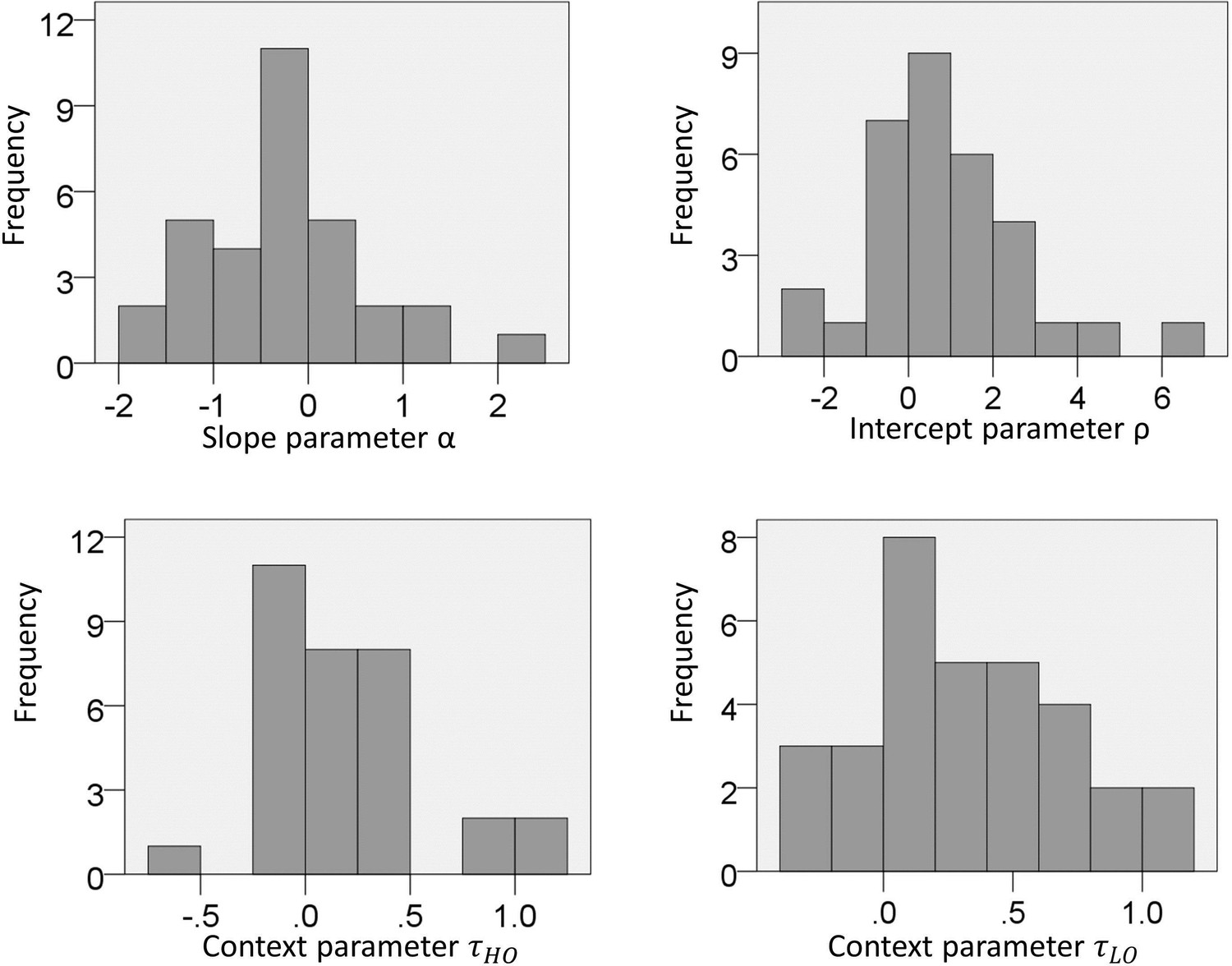
Experiment two: distribution of parameters estimated from choice data with the full model.
https://doi.org/10.7554/eLife.16127.010Additional files
-
Source code 1
Gambling proportion for the different conditions of experiment one.
Rows indicate participants and columns indicate conditions (from left to right: £2, £3, £4, £5 EV in the high-variance context, and £3 and £4 EV in the low variance context).
- https://doi.org/10.7554/eLife.16127.011
-
Source code 2
Data from experiment two. Rows indicate participants and columns indicate data.
The first twelve columns report the gambling proportion for the different conditions (from left to right: HV-deck-set, £9 deck, £11 card; HV-deck-set, £9 deck, £9 card; HV-deck-set, £9 deck, £7 card; HV-deck-set, £7 deck, £9 card; HV-deck-set, £7 deck, £7 card; HV-deck-set, £7 deck, £5 card; LV-deck-set, £7 deck, £9 card; LV-deck-set, £7 deck, £7 card; LV-deck-set, £7 deck, £5 card; LV-deck-set, £5 deck, £7 card; LV-deck-set, £5 deck, £5 card; LV-deck-set, £5 deck, £3 card). Columns 13 and 14 report the average gambling proportion and the effect of card amount on gambling probability (i.e., i.e., the associated regression coefficient of the logistic regression model), respectively. For each deck-set, the difference in gambling between lower and higher value decks for amounts common to both decks (corresponding to £5 and £7 in the low-value deck-set, and to £7 and £9 in the high-value deck-set) was computed and the mean of these two differences is reported in column 15. Column 16 reports the difference in gambling between the low and high value deck-set for the £7 deck (common to both deck-sets).
- https://doi.org/10.7554/eLife.16127.012
Download links
A two-part list of links to download the article, or parts of the article, in various formats.
Downloads (link to download the article as PDF)
Open citations (links to open the citations from this article in various online reference manager services)
Cite this article (links to download the citations from this article in formats compatible with various reference manager tools)
A Bayesian model of context-sensitive value attribution
eLife 5:e16127.
https://doi.org/10.7554/eLife.16127


