A neural basis for the spatial suppression of visual motion perception
- McGill University, Canada
- University of Rochester, United States
Figures
Figure 1
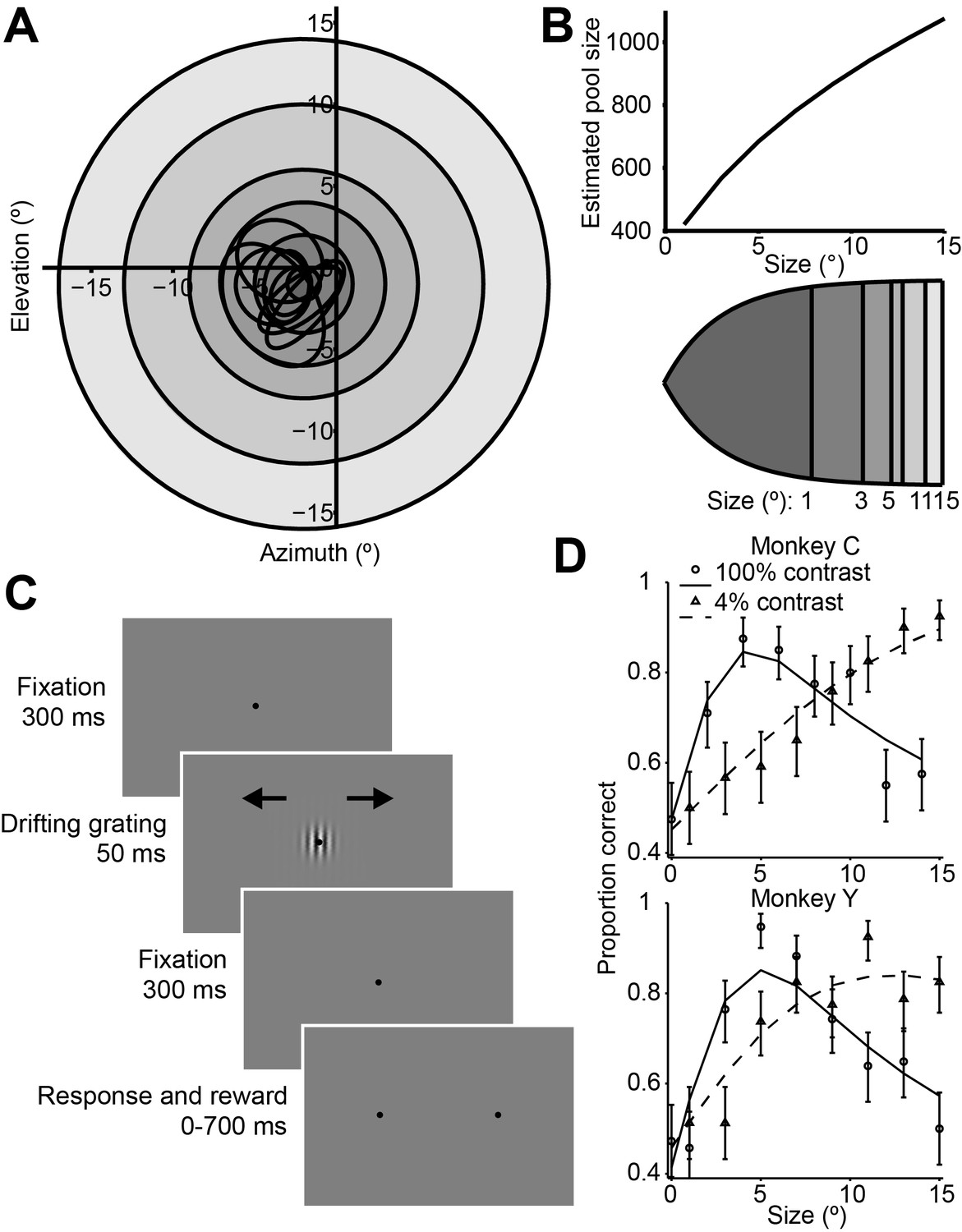
Stimuli, sequence of events, and behavioral performance in the task.
(A) Receptive fields from an example recording session, shown as black ovals, relative to lines of different visual eccentricity (gray circles) commensurate with the stimulus sizes used in the experiments. (B) The estimated neuron pool size as a function of stimulus size, for the eccentricities and stimulus sizes used in the experiments (top). Cortical mapping of visual space from (A), showing that larger stimuli projected onto larger extents of cortical space (bottom). The sizes of the shaded areas correspond to the estimated cortical footprint (see Materials and methods). (C) Behavioral task. The animals were required to maintain fixation in a 2° window for 300 ms, after which a drifting Gabor appeared briefly. Animals were then required to fixate for another 300 ms until the fixation spot disappeared. The animals then indicated their motion percept with an eye movement to one of two targets within 700 ms. (D) Examples of the animals’ psychometric functions for high contrast (solid line, circles) and low contrast (dashed line, triangles) stimuli. Error bars represent 95% binomial proportion confidence interval.
Figure 2 with 2 supplements

Quantification of single neuron selectivity for an example MT neuron, and the summary for the population.
(A) Size tuning curves, plotting the firing rate (mean ± s.e.m.) for the preferred (orange) and null (violet) direction stimuli as a function of Gabor patch size. The lines indicate difference of error functions fits. (B) Neurometric function (filled symbols) for the example neuron plotting the d’ value as a function of stimulus size. The corresponding psychometric function is superimposed (open symbols). Solid and dashed lines indicate difference of error functions fits. The psychophysical performance differs from Figure 1D since the stimulus was tailored to the neural population measured on any one day. (C) Scatter plot of the psychophysical d’ against the neuronal d’ at the largest stimulus size. Filled circles represent monkey C (n = 105), and open squares represent monkey Y (n = 60). Red represents neurons with weak surround suppression, and blue represents neurons with strong surround suppression. The distribution of d’neu-d’psy is shown at the diagonal. (D) The mean d’psy as a function of size from all sessions (monkey C: n = 28, monkey Y: n = 11) superimposed with the mean single neuron d’neu from all MT neurons (165 single neurons). Error bars denote s.e.m. (E) Population summary of choice probability (CP). Scatter plot of CP against the suppression index of the neurometric function. Filled symbols represent CP values that are significantly different from 0.5 (p<0.05, permutation test). Solid line indicates linear fit (r = −0.14, P = 0.04). The marginal distributions of SIneu and CP are shown on the top and the right. Filled and open bars indicate neurons with significant and non-significant choice probabilities, respectively.
Figure 2—figure supplement 1
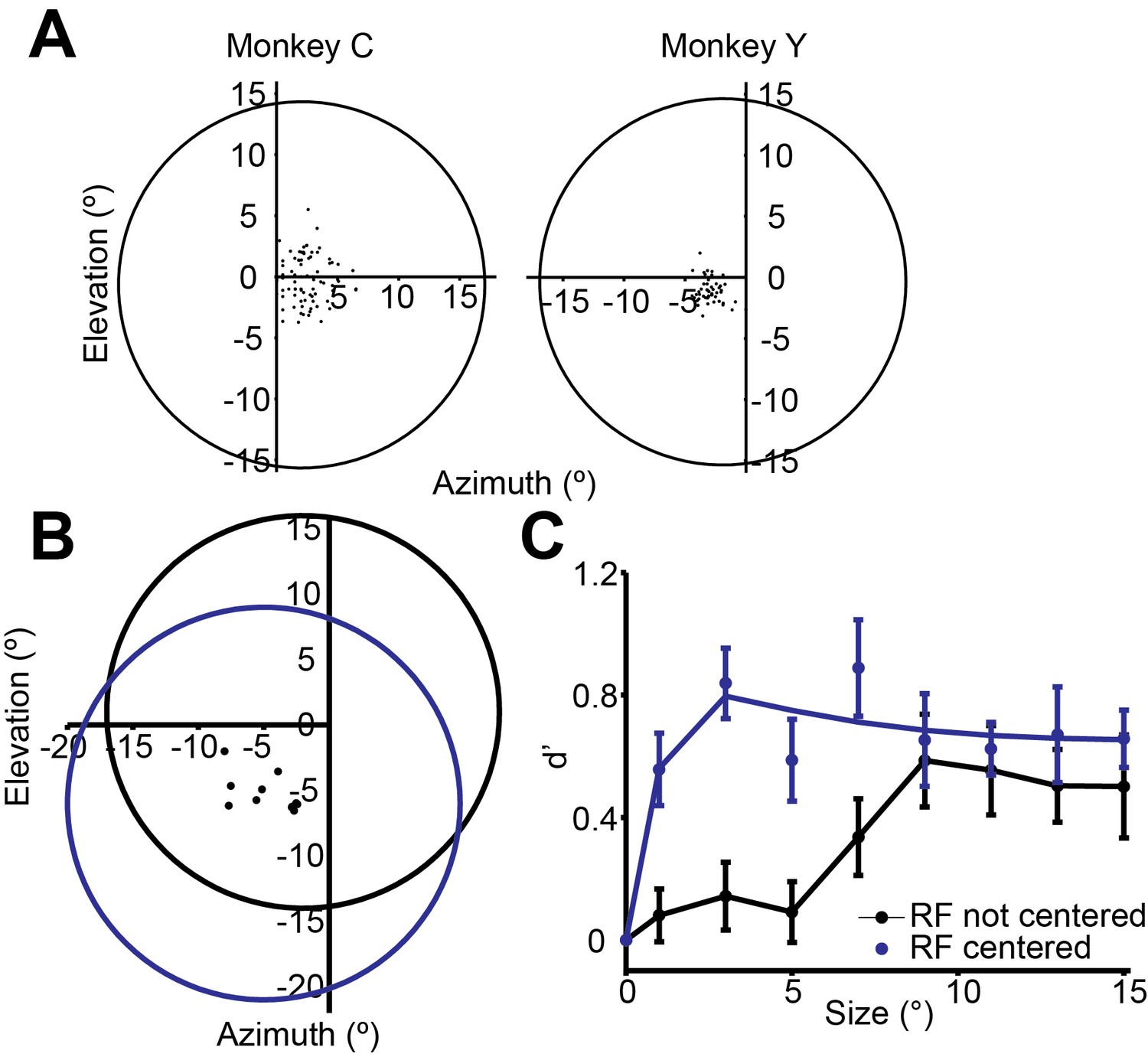
(A) RF positions of the neurons recorded.
The dots are RF centers for the MT neurons from each animal. The circles indicate the average placement of the stimulus centers. Maximal stimulus radius is 15°. The dots represent the centers of the RFs of off-stimulus center neurons simultaneously recorded using the foveal stimulus for the motion direction discrimination task (black circle), and when the stimulus was centered on the RFs (blue circle). (B, C) Single neuron selectivity of peripheral neurons when the foveal stimulus was not centered on the RFs (black), and when the stimulus was centered on the RFs (blue).
Figure 2—figure supplement 2
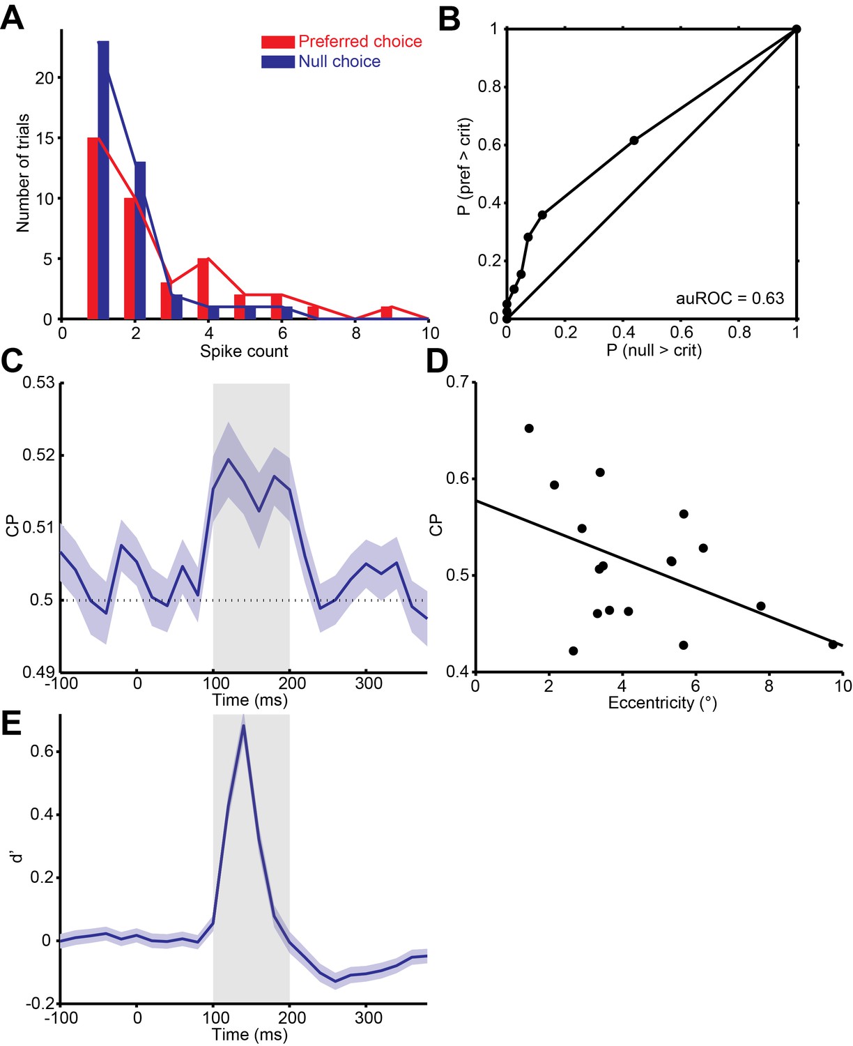
Quantification of choice probability (CP) of single neurons and the time course of CP.
(A) Distributions of firing rates of an MT neuron, grouped according to the monkey’s choice of preferred or null direction motion. (B) The ROC curve of the distributions yielded a significant choice probability of 0.63 (P = 0.010, permutation test). (C) Mean CP across the population was calculated in 20 ms bins. CP was significantly above 0.5 from approximately 100 to 200 ms after stimulus onset (p<0.01, permutation test). (D) Scatter plot of CP against eccentricity of the neurons. Solid line indicates linear fit (r = -0.48, P = 0.05). (E) Mean d’ across the population was calculated in 20 ms bins.
Figure 3
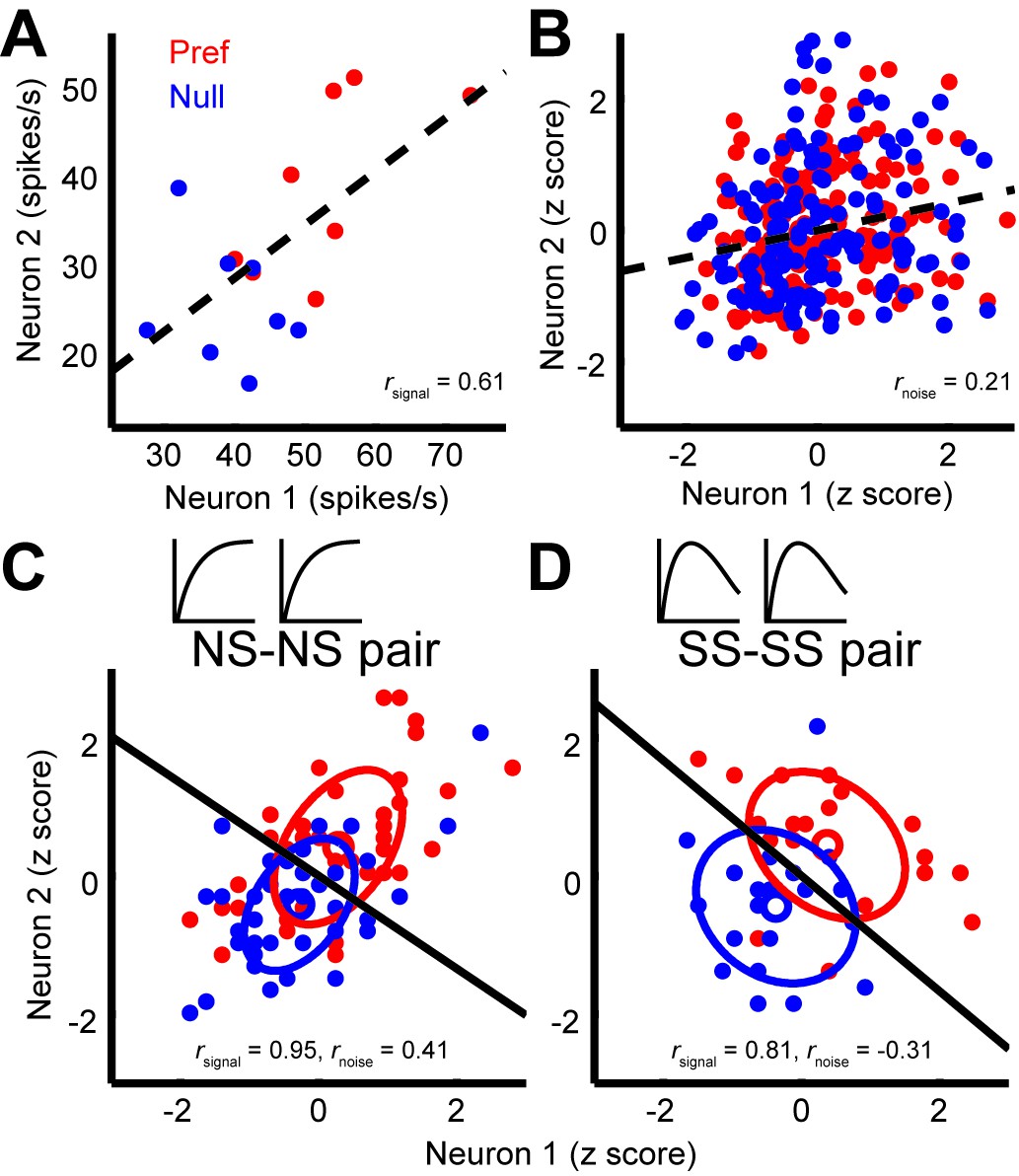
Quantification of noise correlation (rnoise) and signal correlation (rsignal) between neuron pairs.
(A) The mean responses of the two simultaneously recorded neurons across both directions and sizes. rsignal (0.61) is the Pearson correlation coefficient of the mean responses for the conditions. (B) The responses for each stimulus condition were z scored across the repetitions, and each point represents a response from one trial. rnoise (0.21) is the Pearson correlation coefficient of the entire dataset. The dashed lines represent linear fits. (C, D) Response correlations for an NS-NS pair and an SS-SS pair for one example stimulus size (1°).
Figure 4 with 1 supplement
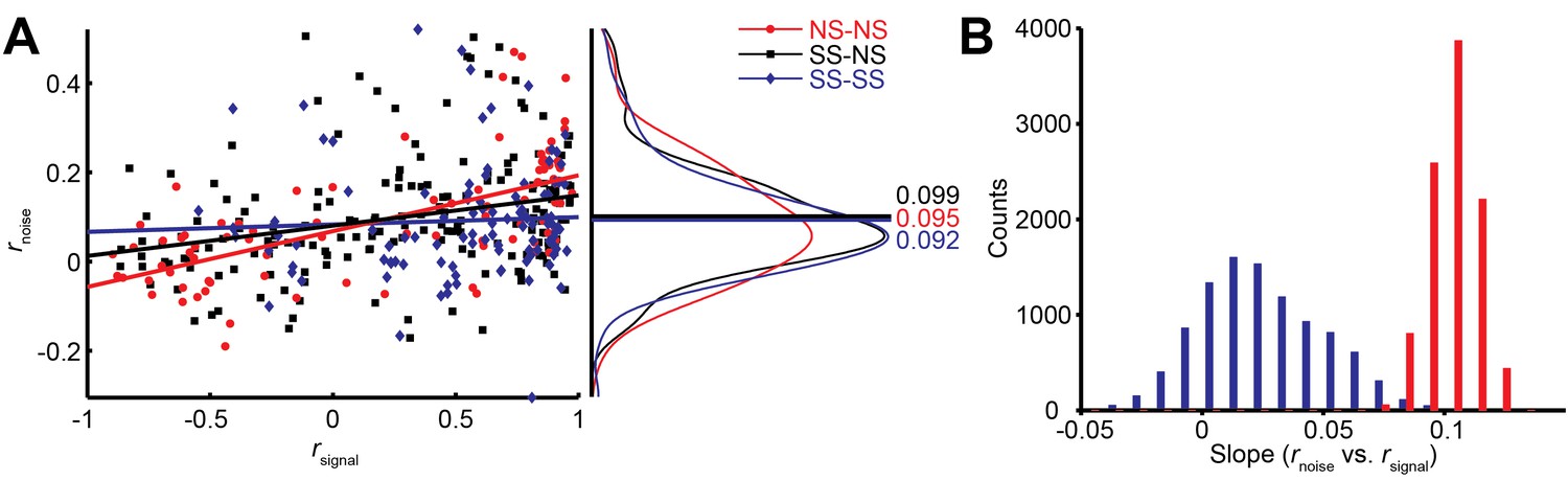
Relationship between noise correlation (rnoise) and signal correlation (rsignal).
(A) Scatter plot of rnoise versus rsignal for pairs of SS and SS (blue), SS and NS (black), and NS and NS (red) neurons. Lines represent linear regression fits. Marginal distributions of rnoise are also shown (right panel). Lines and numbers mark the mean values of rnoise for each combination of neuron pairs. (B) Sampling from rate matched sub-distributions of SS-SS and NS-NS pairs gives similar differences in rnoise vs. rsignal slope.
Figure 4—figure supplement 1
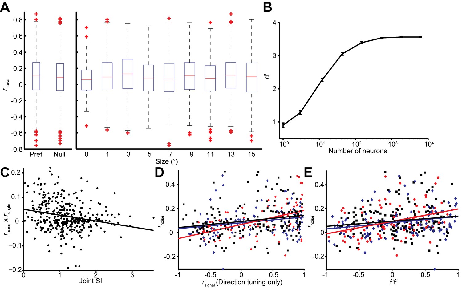
Effects of stimulus conditions, firing rate, and tuning similarity on the rnoise on rsignal dependency.
(A) Box-whiskers plots of the value of rnoise across stimulus conditions. The value of rnoise is not significantly different between the preferred and null directions (Wilcoxon rank sum test, P = 0.07), and smaller and larger sizes (Wilcoxon rank sum test, P = 0.55). (B) Population selectivity as a function of number of neurons included in the simulation. Only the single neuron selectivity at the smallest stimulus size is considered with the mean noise correlation structure observed. (C) The joint SI for each neuron pair (n = 370), determined as the sum of the individual SIs, plotted against the product of rnoise and rsignal for the pair. For the latter, we first subtracted off the mean rnoise and rsignal to isolate the covariance of the two measures. Large positive values correspond to neuron pairs in which rnoise and rsignal have the same sign, as expected for NS-NS pairs (Figure 4A). Small values indicate no consistent relationship between rnoise and rsignal, as expected for the SS-SS pairs (Figure 4A). A linear regression (solid line) confirms a negative relationship between joint SI and the dependency of noise correlations on signal correlations (r = -0.232, p<0.001). (D) A similar rnoise vs. rsignal relationship was observed when rsignal was calculated using separately measured direction tuning curves. (E) A similar rnoise vs. f’f’ relationship was observed when f’ was calculated using the difference between the preferred and null direction responses.
Figure 5 with 4 supplements

Simulation of population selectivity and model comparisons.
(A) Schematic of the population selectivity simulation. The preferred and null responses were sampled from the distribution of parameters recorded. We tested combinations of different correlation structures and readout weights. (B) Calculation of the population selectivity. Each point represents the response from a trial from n neurons (here, n = 2). The one-dimensional distributions for the preferred and null direction responses were generated by projecting the points onto the normalized axis that connects the mean responses in n-dimensional space (factorial read-out). The calculation of population d’ then follows the equation in the Materials and methods. (C) The predicted population neuronal selectivity plotted as a function of the stimulus size for each model. Data points represent averages across 100 iterations of the simulation, with each iteration based on a different re-sampling of the parameter set from the original data sets. Results are shown for the full model based on all empirical measurements in which surround suppression modulates noise correlation structure (cyan); a model where correlations and surround suppression were on average as measured, but the observed relationship between them was missing (magenta), and finally the full model again, but with integration radius of 15° (green). (D) SI of population d’ for simulations where increasing number of neurons with peripheral receptive fields are included. The x-axis indicates the integration window for including neurons’ receptive fields relative to the stimulus center. Error bars denote standard deviation. (E) Comparison of the SI of different simulations: colors as in C. Error bar for the psychophysical data denotes s.e.m., and error bars for the model predictions denote standard deviation.
Figure 5—figure supplement 1
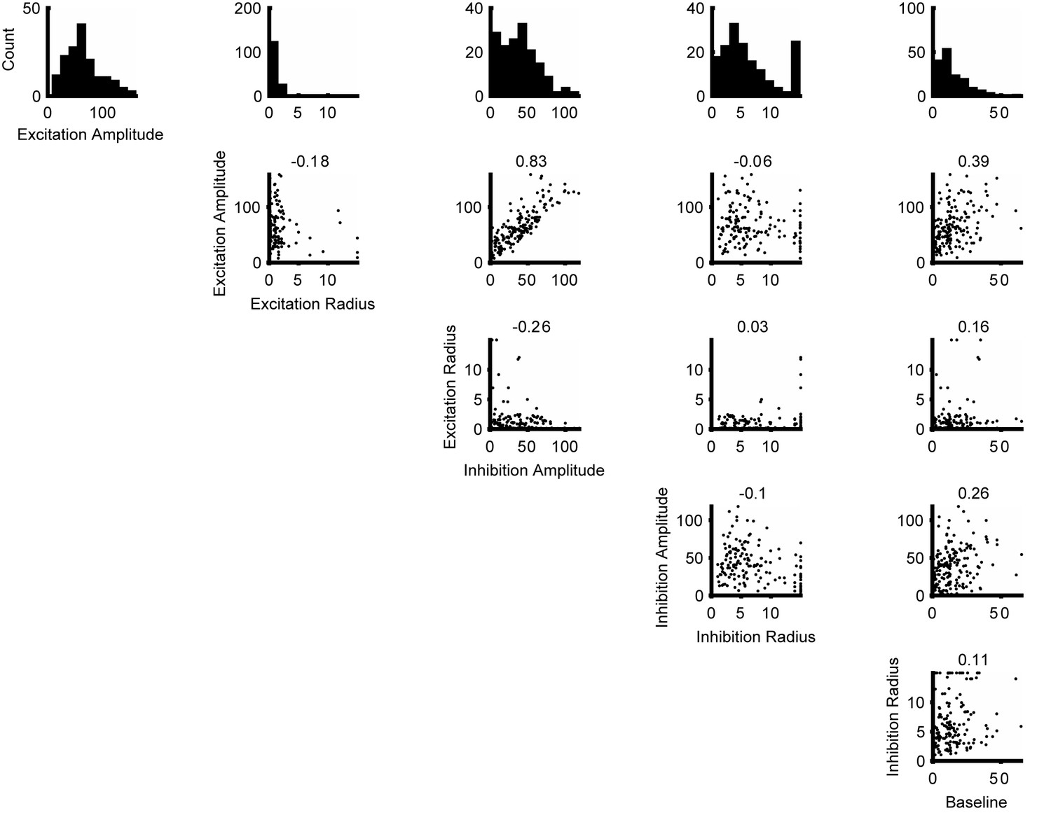
Distributions of the parameters for the Difference of Error functions fits.
The histograms at the top row are the distribution of the parameters. The scatter plots shows the correlation of the parameters. The numbers at the top of each scatter plot are the Pearson correlation coefficients. Together these are used to create a multivariate Gaussian copula that is subsequently truncated to have only positve parameter values.
Figure 5—figure supplement 2
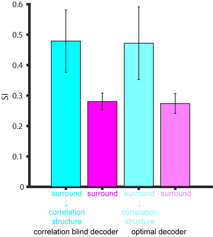
Comparison of the SI of different decoders.
Surround suppression modulation of noise correlation structure (cyan), noise correlation structure with no surround suppression modulation (magenta) from Figure 5E using the factorial versus optimal decoders. Error bars denote standard deviation.
Figure 5—figure supplement 3
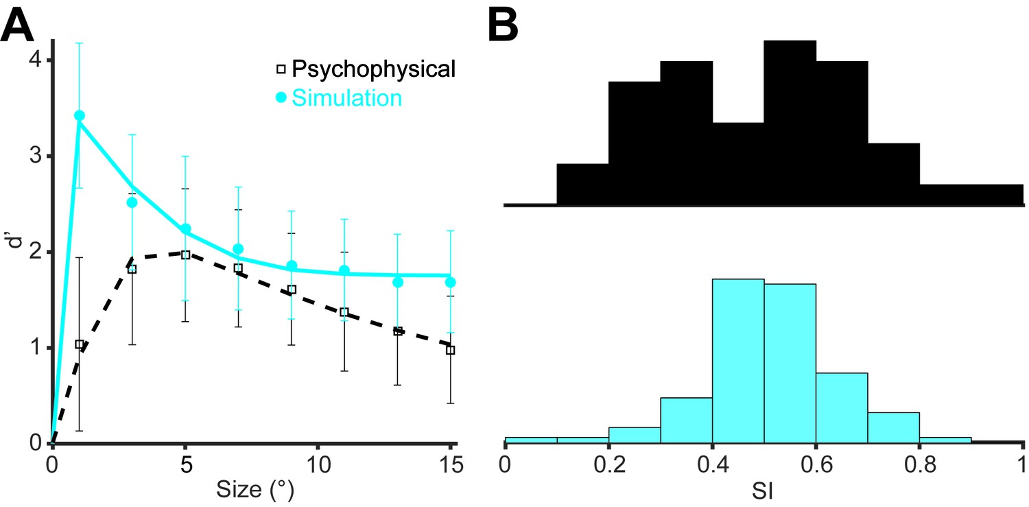
Distributions of measured and simulated behavioral d’ and SI.
(A) The d’ values plotted as a function of the stimulus size. Data points represent averages across 39 psychophysical measurements (black) and 100 simulations (cyan). Error bars denote standard deviation. (B) Distributions of SIs for the same psychophysical measurements (black) and simulations (cyan).
Figure 5—figure supplement 4
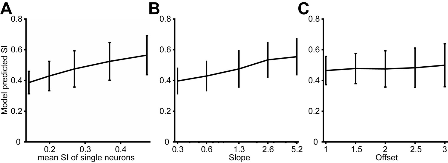
Predicted model SI as other model parameters were varied.
(A) The predicted model SI when single-neuron SI is adjusted. The x-axis indicates the average SI of single neurons. (B) The predicted model SI when the slope of the relationship between correlation and surround suppression is varied. The offset was fixed at 2. (C) The predicted model SI when the offset of this relationship is varied. The slope was fixed at 1.3. Error bars denote standard deviations across 100 simulations in all plots.
Download links
A two-part list of links to download the article, or parts of the article, in various formats.
Downloads (link to download the article as PDF)
Open citations (links to open the citations from this article in various online reference manager services)
Cite this article (links to download the citations from this article in formats compatible with various reference manager tools)
A neural basis for the spatial suppression of visual motion perception
eLife 5:e16167.
https://doi.org/10.7554/eLife.16167


