Stacking the odds for Golgi cisternal maturation
Figures
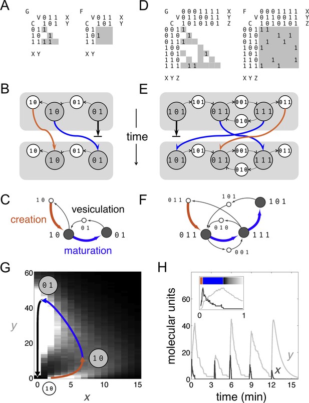
Boolean dynamics of compartments and vesicles: examples of maturation chains.
(A,B,C) A system with molecular labels X and Y. (D,E,F) A system with molecular labels X, Y and Z. (A,D) Left: the budding matrix = 1 means compartment type i (row) buds out vesicle type j (column). Vesicle compositions are subsets of source compartment compositions, so only some entries of can be non-zero (gray shading). Right: the fusion matrix = 1 means vesicle type j (column) can fuse with compartment type i (row). Any entry of can be non-zero (gray shading). (B,E) At each timepoint compartments (gray circles) accept (through fusion) or give away (through budding) vesicles (white circles). Gray rectangles show the state of the cell at successive timepoints, moving from top to bottom. Compartments can undergo maturation (blue arrows) or vesiculate by giving up all their cargo (thick black arrows); orphan vesicles can undergo homotypic fusion to generate new compartments (brown arrows). From the first to the second timepoint, individual compartments change composition but the full set of compartments is constant: the system has reached homeostasis. (C,F) Another representation of the homeostatic networks from Figure 1B,E, mapping out a cell in compositional space. Circles represent compartments (gray) or vesicles (white); each distinct circle represents a distinct compositional type. Thin black arrows show vesicles moving between compartments at one timepoint. Brown arrows followed by blue arrows show the creation and maturation of compartments, flowing from one timepoint to the next. (G,H) Results of a stochastic simulation of vesicle traffic for a system with two molecular labels X and Y (Box, Equation 1). The cell contains many vesicles and compartments, and reaches an equilibrium in which the vesicle pools and the number of compartments of each compositional type are approximately constant. Parameters: = {250 units, 5000 units}; {A, B, C, D} = {1000 units min−1, 10 min−1, 5 min−1, 1 min−1}; time-averaged vesicle pools , . Timescales are chosen to qualitatively match real maturation dynamics (Losev et al., 2006). (G) The heatmap shows the equilibrium distribution of compartment compositions. Individual compartments change composition over time: the curve shows the deterministic limit-cycle solution to Equation 2, with different phases corresponding to creation (brown), maturation (blue), and vesiculation (black). Extrema of this curve correspond to the Boolean compartment compositions in Figure 1C. (H) Compositions of individual compartments over time for the full stochastic simulation (X in dark gray, Y in light gray). Compositions cycle periodically; each cycle is independent of the previous one, since new compartments are nucleated by fresh homotypic fusion events. The final cycle shows the deterministic limit-cycle solution to Equation 2 for comparison. The inset expands the first minute, with X and Y levels scaled against their maximum values so creation, maturation and vesiculation can be clearly observed. Figure 1—figure supplement 1 shows how non-vesicular transport can be included in this framework.

Combining vesicular and non-vesicular transport.
Example of a system with molecular label types. The Rab GTPase (R) shuttles between the cytoplasm and the membrane. The GDF (D: GDI displacement factor) recruits the Rab GTPase to the correct membrane. The GEF (E: GDP/GTP exchange factor) converts the Rab to its active GTP-bound form. The GAP (A: GTPase activating protein) coverts the Rab to its inactive GDP-bound form, which moves to the cytoplasm. We show two sets of Rabs and their regulators, in red and green. In addition, we track membrane lipids that move along vesicles (M) in blue. Left: the budding and fusion matrices and . There are possible types of compartments and vesicles, we only show a subset of them here. Rabs, GEFs and GAPs moving through the cytoplasm are represented just as vesicles are, but with a single label and lacking membranes. Right: homeostatic vesicle traffic systems corresponding to the budding and fusion rules. Compartments are shown as large gray circles, vesicles are explicitly shown as small white circles, non-vesicular transport pathways are shown as arrows between compartments. (A) Rab-mediated vesicle exchange between two distinct compartments. (B) A Rab GTPase cascade. The active form of one Rab recruits its own GAP, but recruits the other Rab’s GEF. This causes a single compartment to oscillate between the two Rab varieties, shown as a maturation cycle (blue arrows). This is similar to the Rab5/Rab7 switch during endosomal maturation (Rink et al., 2005).
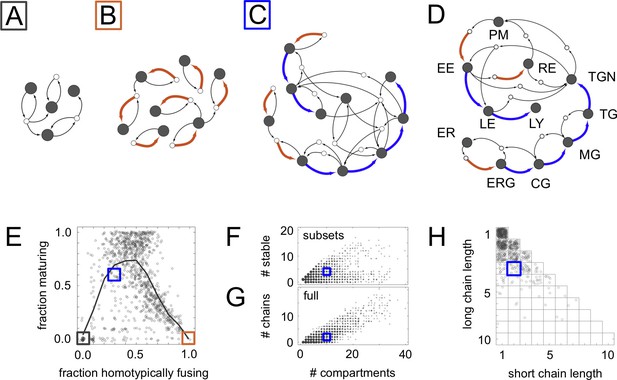
Homeostatic vesicle traffic networks.
These data relate to the 14,809 homeostatic networks for molecular label types. (A–C) Examples of homeostatic networks (compartment and vesicle compositions are omitted for clarity) for budding and fusion rules generated using different parameter values (Materials and methods: Sampling homeostatic vesicle traffic networks). (A) {7, 1, 0.35, 0.35}, gray square icon. This is a transport-balanced network with no homotypic fusion or maturation. (B) {7, 4, 0.025, 0.75}, brown square icon. This is a network with high homotypic fusion but no maturation, and is broken into many disconnected subsets. (C) {7, 2, 0.1, 0.7}, blue square icon. This network has low homotypic fusion and high maturation, similar to a real eukaryotic cell. (D) Schematic vesicle traffic system of a eukaryotic cell. ER: endoplasmic reticulum. ERG: ER-Golgi intermediate compartment. CG: cis-Golgi. MG: medial-Golgi. TG: trans-Golgi. TGN: trans-Golgi network. PM: plasma membrane. EE: early endosome. LE: late endosome. LY: lysosome. RE: recycling endosome. (E) For each network in our dataset with ten or more compartments, we show the fraction of compartments undergoing maturation (outgoing blue arrow) vs. the fraction of compartments created by homotypic vesicle fusion (incoming brown arrow). The gray curve shows a moving average of the data. The colored squares show the position of the three networks in Figure 2A–C. Maturation is most likely at low-to-moderate rates of homotypic fusion. (F) The number of stable compartments vs. the total number of compartments for all the connected subsets in our dataset. The ER and plasma membrane are examples of stable compartments in real cells. (G) The number of maturation chains vs. the total number of compartments for all the networks in our dataset. (H) Chain lengths for all 841 networks in our dataset with precisely two maturation chains. In (E–H) we plot values with a random additive noise so the density of points can be observed. The blue square icon shows the properties of the cell-like network from Figure 2C. Figure 2—figure supplements 1,2 explore further properties of these homeostatic networks.
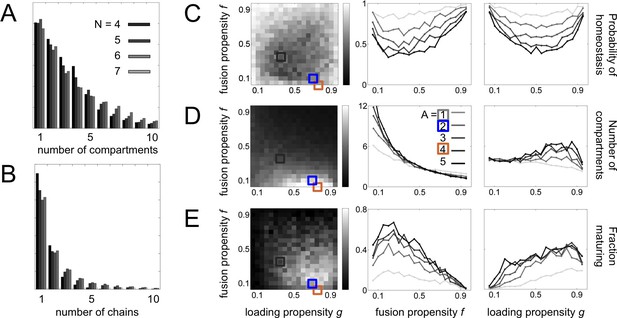
Statistical sampling of networks.
(A,B) For systems with molecular label types, we show the histogram of (A) the number of compartments and (B) and the number maturation chains. There is almost no variation when going from to label types. (C,D,E) Properties of systems for label types and adaptor/coatomer types; A sets the limit on the number of distinct vesicles a compartment can generate. We generate random budding and fusion matrices using two parameters (Materials and methods: Sampling homeostatic vesicle traffic networks): g is the loading propensity of molecular labels onto vesicles; f is the fusion propensity between vesicles and compartments. For each combination of parameters we generate ten sets of matrices G and F. For each instance of G and F we run the vesicle traffic dynamics starting from a random initial condition. We store all homeostatic states resulting from this procedure, and track the average value of any property across them. (C) Probability of reaching a homeostatic steady state from a random initial condition. (D) Number of compartments. (E) Fraction of compartments involved in a maturation process. Left column: the relevant quantity as a heat map for fixed g and f, but any A. Middle and right columns: the relevant quantity for each value of A, as a function of fixed f (middle) or fixed g (right). The adaptor/coatomer number A weakly influences the number of compartments, but strongly influences the fraction of compartments undergoing maturation. The gray, brown and blue square icons show the parameters used to generate of the networks from Figure 2A–C.

Properties of homeostatic networks.
These data relate to the 14,809 homeostatic networks for molecular label types. (A) The homeostatic networks generated by our sampling procedure can break into subsets of compartments connected within themselves but mutually disconnected from one another. (In graph theory these would be called 'connected components'; we use the term 'subsets' to avoid confusion with molecular components.) The diagonal shows the trivial networks where each compartment is disconnected from all the others, so the number of subsets is equal to the number of compartments. The horizontal line above the x-axis shows the completely connected networks consisting of a single subset. (B,C) The number of vesicles vs. the number of compartments for (B) all networks, and (C) connected network subsets. (D) Histogram showing the number of molecule types on compartments (top) and vesicles (bottom). (E) Any group of compartments for which some molecule type flows in but not out corresponds to a sink, and implies the need for compensatory synthesis at long timescales. Here we show the number of molecules with sinks vs. the total number of compartments, for all connected subsets in our dataset. The gray curve shows a moving average. (F,G) The fusion (F) and budding (G) matrices used to generate the cell-like network from Figure 2C. Non-zero entries are shown as black pixels. (H) The flow of molecules in the cell-like network from Figure 2C. The path taken by each of the molecular label types are separately highlighted. The network is homeostatic with respect to composition but not quantity. Some molecules move in cycles while others (the first and the third in this example) have sinks and therefore require compensatory synthesis.
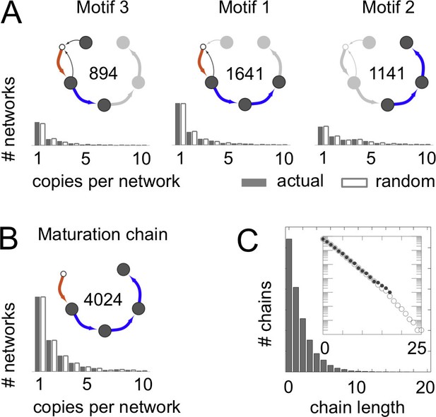
Frequent vesicle traffic motifs.
These data relate to the 14,809 homeostatic networks for molecular label types. (A,B) Insets indicate the number of homeostatic networks that contain at least one copy of the motif. Histograms show the number of repeated copies of each motif per network, in actual (gray bars) or randomized (white bars) networks (Materials and methods: Vesicle traffic motifs; Materials and methods: Randomly shuffled vesicle traffic networks). (A) The three most frequent connected three-compartment motifs. (B) The maturation chain. (C) Histogram of maturation chain lengths. We consider any compartment with an incoming brown arrow as the start of a chain, and define length as the number of subsequent blue arrows. Inset: the same data in a log-linear plot. Both the real (grey dots) and randomized (white dots) networks show a geometric distribution of chain lengths. Figure 3—figure supplement 1 shows the frequency of the top 100 most common motifs.
Vesicle traffic motif statistics.
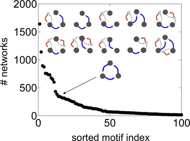
The number of networks in which each connected 3-compartment motif occurs vs. the motif index (Materials and methods: Vesicle traffic motifs). Motifs are sorted along the x-axis, from most to least frequent. The insets show the top 10 most frequent motifs (first two rows). We also show the 15th most common motif: the maturation cycle.
Anatomy of a cisternal maturation chain.
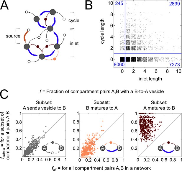
(A) A compartment created at the first timepoint (source, thick brown arrow) matures at each successive timepoint (inlet, thick blue arrows). This process can terminate at a compartment with fixed composition, or one with an oscillating composition (cycle of thick blue arrows). Vesicles move molecules between compartments. We classify vesicles as anterograde (thin light brown arrows), retrograde (thin dark brown arrows) and other (thin black arrows). Some vesicles are inbound or outbound from other parts of the network. (B) Properties of the terminal compartment of a maturation chain. There are 10,172 homotypically fusing sources in our dataset that have at least one maturation step, of which just 2899 terminate in a cycle. The remaining 7273 sources terminate at 4588 fixed compartments (the reduction in number is because maturation chains can converge). Finally, 2820 of these 4588 compartments dissipate at the next timestep, giving up all their cargo as vesicles. (C) Fraction of compartment pairs A,B with a B-to-A vesicle. Each dot in each panel represents values for a single network; we show data only for networks that have ten or more maturation edges. The x-axis is the vesicle fraction for all compartment pairs A,B in the network. The y-axis is the vesicle fraction for the subset of compartment pairs A,B in the network where A sends a vesicle to B (left), B matures to A (middle), or A matures to B (right). For the left and middle panels, the chance of finding a B to A vesicle for the corresponding subset of pairs is the same as the chance between all pairs in a network. For the right panel, the chance of finding a B to A vesicle when A matures to B (median 0.75) is eight fold more than the chance across all pairs (median 0.09). For example, suppose a network with 10 compartments has compartment pairs A,B. Suppose for 8 of these pairs we know that A matures to B. Now we count vesicles. We find that 8/90 = 0.09 of all pairs and 6/8 = 0.75 of the maturing pairs have a vesicle going from B to A. This corresponds to a network with an x-value of 0.09 and a y-value of 0.75: there are many more retrograde vesicles between maturing compartments than expected by chance. That is, a younger compartment in a maturation chain almost certainly receives a retrograde vesicle from its immediate older successor. Figure 4—figure supplement 1 explores the optimal spatial distribution of compartments in a maturation chain.
Spatial optimization of networks.
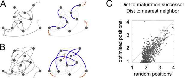
We optimize the spatial locations of compartments such that all parts of a cell are close to at least one compartment, while the distance travelled by vesicles between compartments is minimized (Materials and methods: Spatial optimization). (A,B) The cell-like network from Figure 2C. Maturation chains line up spatially, so each compartment is adjacent to the compartment type it matures to. This is reminiscent of Golgi stacks in real cells. Left panels: the network showing vesicle arrows alone, which are the inputs used for optimization. Right panels: the network showing creation and maturation arrows, with maturation chains clearly forming stacks. (A) The optimized network. (B) The network with compartment identities randomly shuffled, shown for comparison. (C) Effect of optimization across all networks with ten or more compartments. For each network, we plot the mean pairwise distance between compartments connected by blue maturation arrows, scaled by the nearest neighbor distance. The x-axis shows the distances for randomly shuffled networks, the y-axis shows the optimized distances. Though the optimization protocol only considers vesicle arrows and is ignorant of maturation arrows, the distance between compartments in a maturation chain is dramatically reduced. 42% of optimized networks have a mean distance of less than 1.5, while no random networks do.


