Attention operates uniformly throughout the classical receptive field and the surround
- The University of Chicago, United States
- Harvard Medical School, United States
- Katholieke Universiteit Leuven, Belgium
Figures
Figure 1
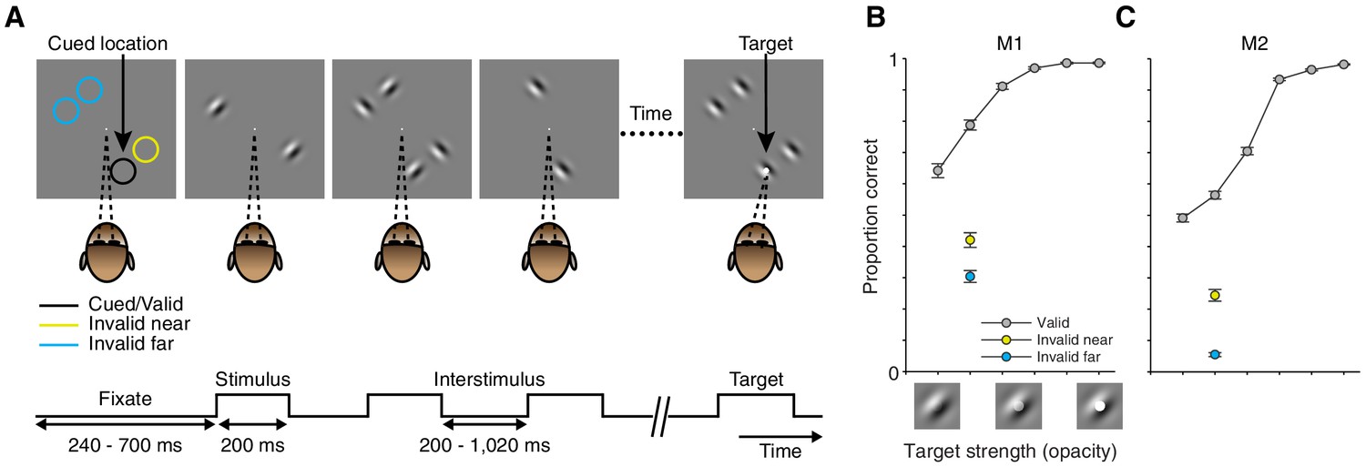
Task and performance.
(A) Every trial consisted of a sequence of stimulus presentations. On each stimulus presentation (200 ms duration; 200–1020 inter-stimulus interval), Gabor stimuli of two orthogonal orientations could be presented at four possible stimulus locations. The monkey was rewarded for detecting a faint white spot (target) in the center of one Gabor during one stimulus presentation. For 91% of trials the target was presented at the cued location (location of the black circle; valid trials). On the remaining 9% of trials the target was presented at one of three uncued locations: adjacent to the cued location (location of the yellow circle; invalid near), or at one of two locations on the opposite side of the fixation point (location of the blue circles; invalid far). Colored circles in (A) are shown for illustrative purposes, never presented during the task. (B) Average performance across recording sessions for monkey M1. Proportion correct (± SEM based on N = 52 sessions; proportion correct at equal target strength: Valid: 0.79; Invalid near: 0.42; Invalid far: 0.30) as a function of target strength for trials in which the target occurred at the cued (gray: valid) or uncued (yellow: invalid near; blue: invalid far) location. Target strength is defined as the opacity of the target. The pictograms below the target-strength axis illustrate the nature of the target-strength manipulation but do not represent actual target-strength values used during the recordings. (C) Average performance across recording sessions for monkey M2 (N = 78 sessions; proportion correct at equal target strength: Valid: 0.56; Invalid near: 0.24; Invalid far: 0.05).
Figure 2 with 1 supplement
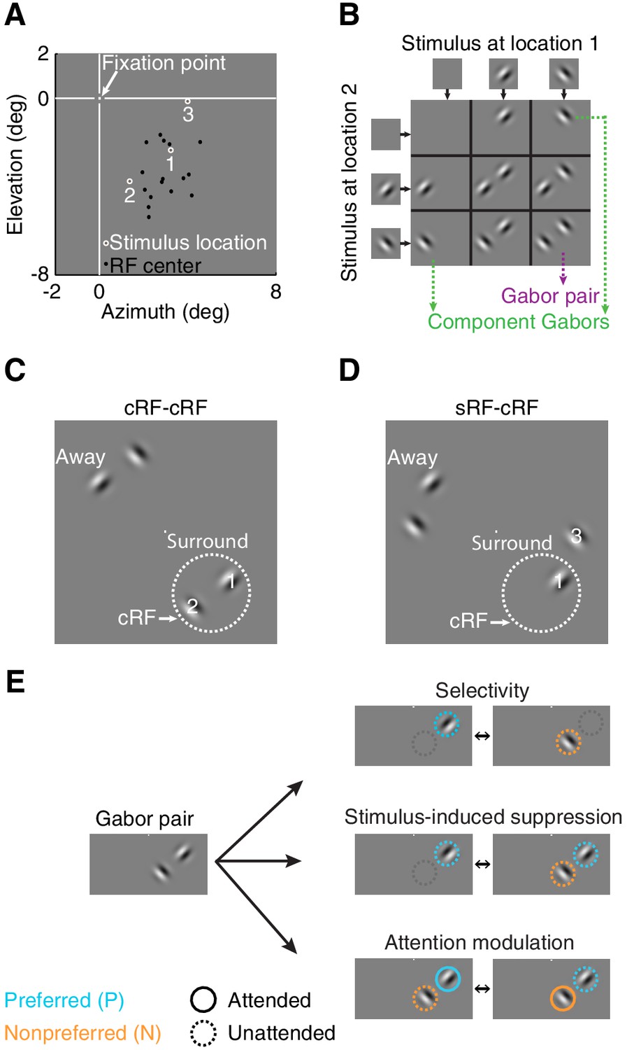
Stimulus conditions.
(A) Neurons' receptive field centers were located in the lower right visual field: black dots indicate receptive-field centers of 16 simultaneously recorded neurons from one recording session. White circles (1,2,3) indicate the three stimulus locations near the neurons' receptive field for this example session. Within a block of trials, only two stimulus locations were used: locations 1+2 or 1+3. (B) Nine possible stimulus combinations resulting from two stimulus locations and two orthogonal orientations. (C) Two receptive-field configurations: cRF-cRF stimulus configuration with two stimuli inside the neuron's classical receptive field. White dotted circle illustrates the cRF. (D) sRF-cRF stimulus configuration with one stimulus inside a neuron's cRF and an adjacent stimulus in its surround. Each stimulus location near the neurons' receptive fields (stimulus location 1,2,3 in 2A) had a corresponding stimulus location on the opposite side of the fixation point (stimuli near Away in C, D; see also Figure 2—figure supplement 1). (E) Pictograms illustrate for one Gabor pair the stimulus configurations used to calculate all indices. Cyan circles indicate the preferred Gabor (P), orange circles the non-preferred Gabor (N). Solid circles represent task conditions wherein attention was directed toward a stimulus location near the neurons' receptive field (PAttN, PNAtt). Dashed circles indicate that the stimulus was unattended and attention was directed toward another location.
Figure 2—figure supplement 1
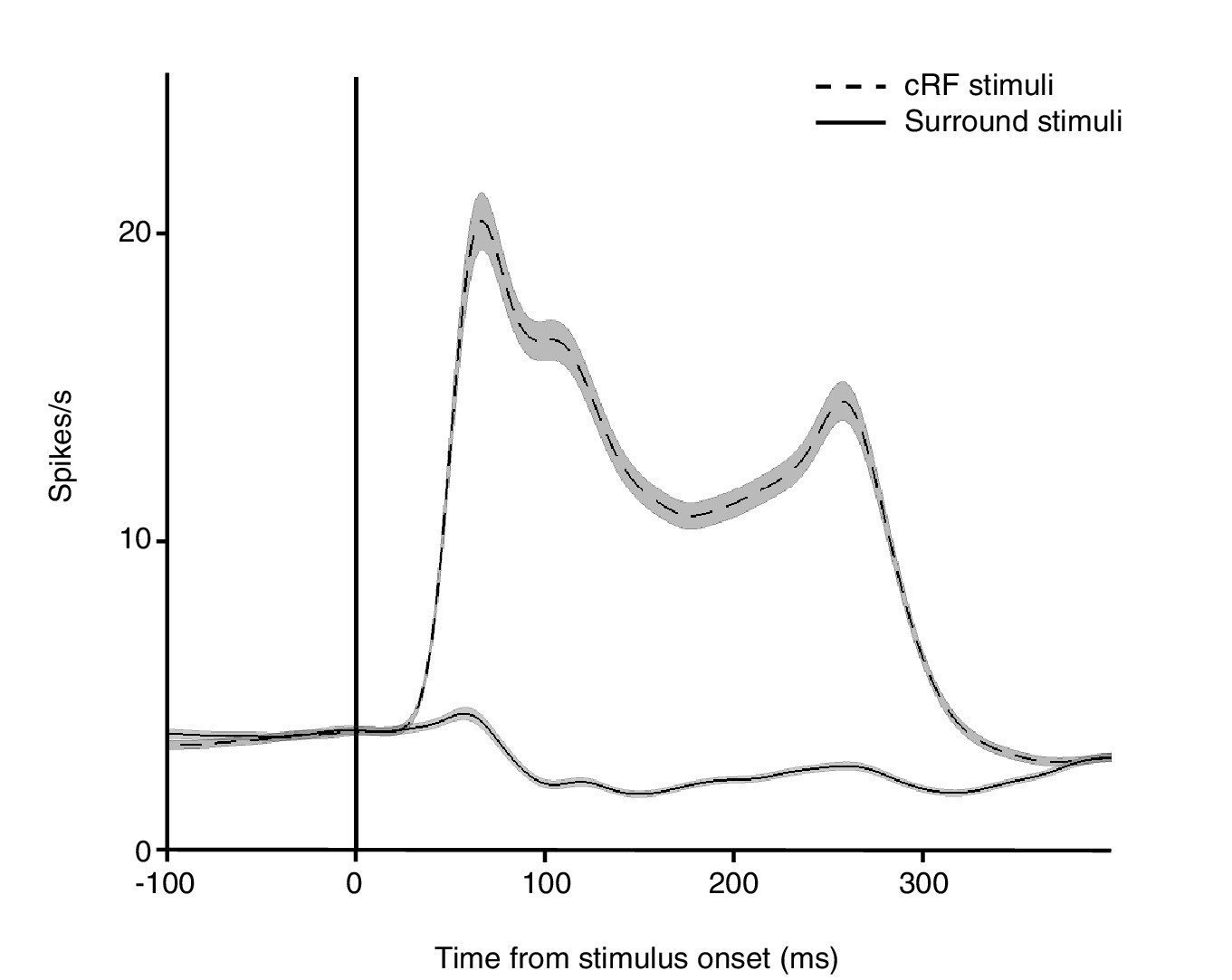
Average PSTH for individual Gabor stimuli presented inside the classical receptive field (cRF) and within the surround.
Shown are the average responses from the same V4 neurons to a Gabor stimulus placed either inside the cRF (dashed line) or within the surround (solid line). Surround stimuli on average slightly suppressed the baseline response. Black vertical line indicates stimulus onset. Shading over the lines indicates ± SEM. Based on the responses from 558 neurons for which a surround position was examined.
Figure 3

Example attention modulations.
Responses of four different neurons to a selected Gabor pair are shown (measured in different sessions). (A) Example 1: cRF-cRF configuration. Left panel shows this neuron's receptive-field map with the two stimulus locations at which the Gabors were presented overlaid (white-gray dots). Right panel PSTHs show the neuronal responses to the Gabor pair when attention was directed toward the preferred Gabor (cyan line; PAttN), the non-preferred Gabor (orange line; PNAtt), or a stimulus on the opposite side of the fixation point (green dashed line; PN; attend away). Bar-plot inset shows the responses of this neuron to a Gabor pair (PN) and its component Gabors (P, N), all measured in the attend away condition. This neuron's response was selective to the component Gabors of the Gabor pair (P vs. N), suppressed by the addition of a non-preferred Gabor to a preferred Gabor (P vs. PN), and strongly modulated when attention was shifted between the two component Gabors of the Gabor pair (PAttN vs. PNAtt). (B) Example 2: another neuron in the cRF-cRF configuration. This neuron showed weak selectivity, hardly any suppression, and little attention modulation. (C) Example 3: sRF-cRF configuration with one Gabor inside the neuron's cRF, and one Gabor inside its surround. By definition, the cRF Gabor is preferred (P) and the silent surround Gabor is non-preferred (N). The neuron responded highly selectively to the cRF and the surround Gabor when presented alone (P vs. N), showed surround suppression (P vs. PN), and was modulated by attention (PAttN vs. PNAtt). (D) Example 4: another neuron in the sRF-cRF configuration. This neuron was highly selective to the component Gabors of the Gabor pair, but only weakly suppressed by the surround Gabor, and showed little attention modulation. The insets show the average waveforms of the recorded neurons (blue) plus that of the multi-unit activity measured at the same electrode (grey). Shading around the mean represents ± 2 median absolute deviation (MAD). Scale bars indicate 50 μV and 0.1 ms. The receptive-field maps were normalized to the maximum response for each neuron during receptive-field mapping (RF max), dark blue shows the baseline response. Error bars represent ± SEM.
Figure 4 with 1 supplement
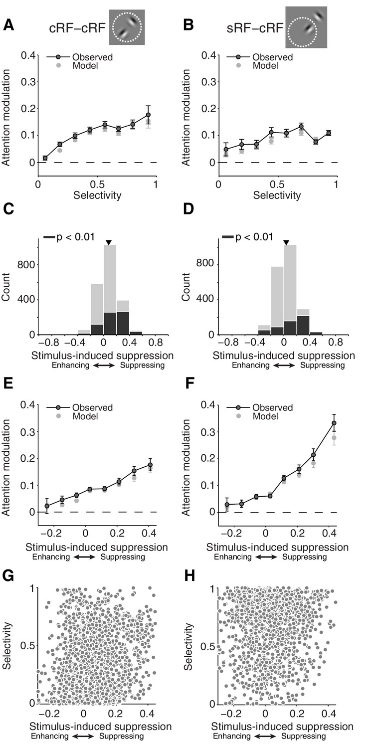
First-order analyses suggest that attention modulation follows different principles for stimuli inside the cRF and the surround.
(A, B) Average attention modulation as a function of the stimulus selectivity in the cRF-cRF and sRF-cRF configuration respectively. Low selectivity occurs in the sRF-cRF configuration when neurons respond weakly to the cRF stimulus, e.g. because of a non-preferred orientation or a weakly responsive cRF location, and have a baseline response to the surround stimulus. (C, D) Histogram of all stimulus-induced suppression indices measured in the cRF-cRF and sRF-cRF configuration respectively. The suppression index is negative when neurons increase their response when a non-preferred stimulus is added to the preferred stimulus (enhancing), and positive when neurons decrease their response when a non-preferred stimulus is added to the preferred stimulus (suppressing). Black bars indicate indices associated with Gabor pairs for which the suppression index differed significantly from zero (p<0.01; permutation t-test; see also Figure 4—figure supplement 1). Triangle points to the mean suppression index. (E, F) Average attention modulation as a function of stimulus-induced suppression in the cRF-cRF and sRF-cRF configuration respectively. Error bars represent ± SEM. (G, H) Stimulus-induced suppression versus stimulus selectivity for all Gabor pairs in the cRF-cRF (N = 1769) and sRF-cRF (N = 1768) configuration respectively.
Figure 4—figure supplement 1
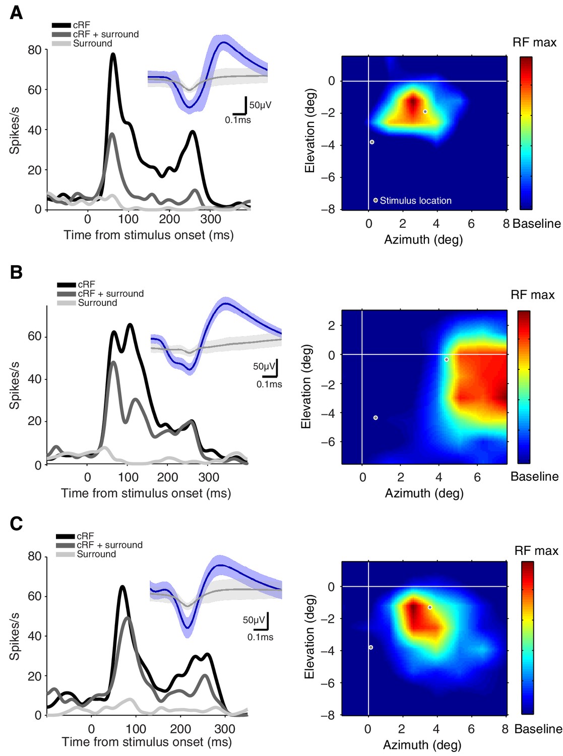
Example neurons with strong surround suppression.
A, B, C three neurons with significant surround suppression (p<0.01). The left panels show the average responses of the neurons to single stimuli presented either inside the cRF (black; cRF), the surround (light grey; Surround) and the responses to the combined presentation of both the cRF and the surround stimulus (grey; cRF + surround). The insets show the average waveforms of the recorded neurons (blue) plus that of the multi-unit activity measured at the same electrode (grey). Shading around the mean represents ± 2 median absolute deviation (MAD). The right panels show each neuron's receptive-field map with the two stimulus locations at which the Gabors were presented overlaid (white-gray dots). The receptive-field maps were normalized to the maximum response for each neuron during receptive-field mapping (RF max), dark blue shows the baseline response. See Figure 3C for another example.
Figure 5 with 1 supplement
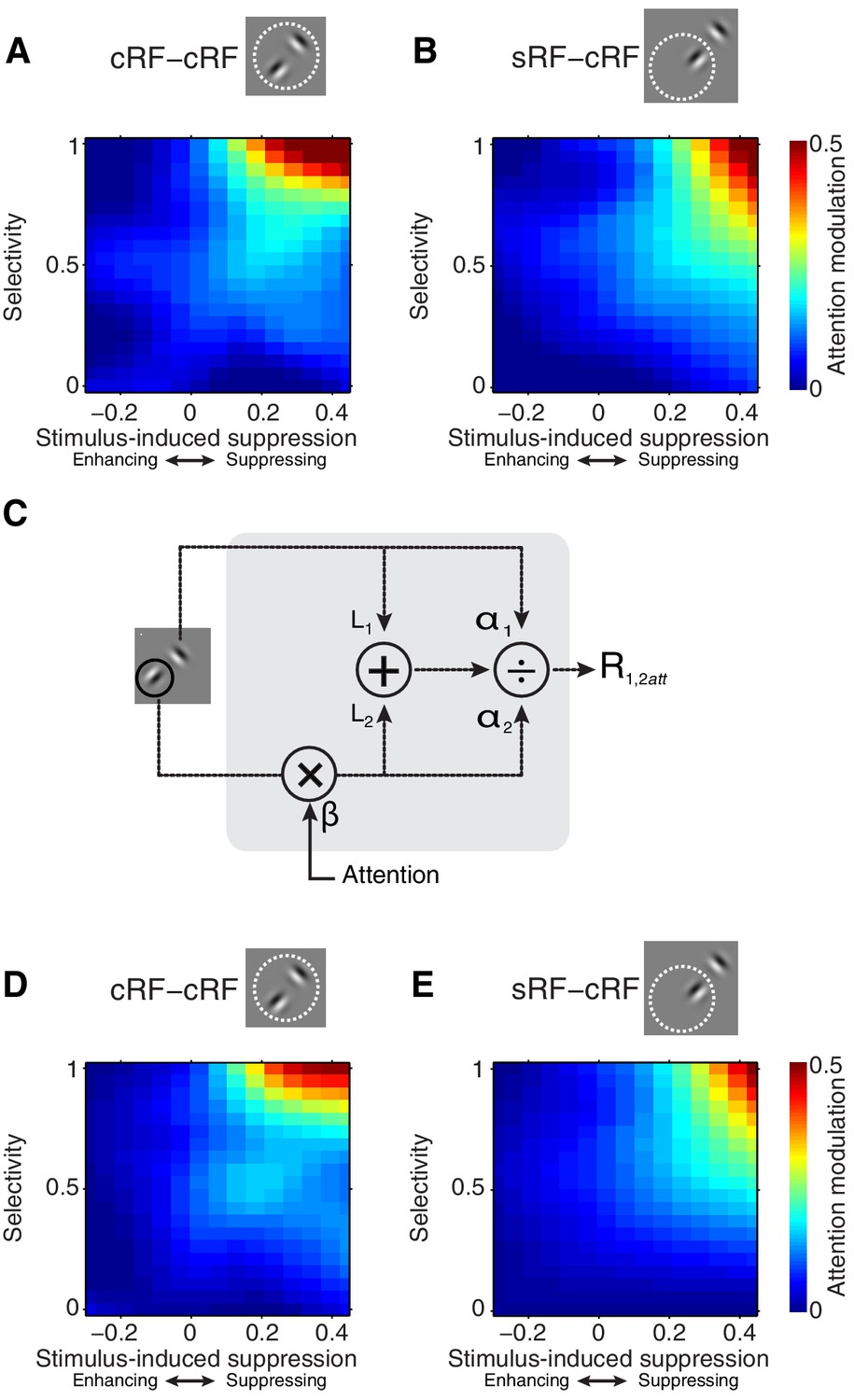
Selectivity and stimulus-induced suppression interact to control attention modulation.
(A, B) Average attention modulation as a function of stimulus-induced suppression (x-axis) and stimulus selectivity (y-axis) in the cRF-cRF and sRF-cRF configuration respectively. The magnitude of attention modulation is indicated by color (red = strong, blue = weak). Note that, although the data covered most of this space (see Figure 4G,H), few regions, e.g. the lower right corner in (B), were not well sampled. (C) Model schematic. Every stimulus contributes an excitatory drive (L1 and L2) to the neuron's response (R1,2att) to a Gabor pair. Each stimulated receptive-field location, either inside the cRF or inside the surround, contributes divisive suppression (α1 and α2) to the neuron's response. The divisive suppression is fixed for each receptive-field location, independent of the stimulus presented at that location. A small amount of baseline suppression is further added (σ parameter; not shown). Directing attention toward a stimulus location has a multiplicative effect (β) on the parameters (L2 and α2) corresponding to the attended receptive-field location (location 2 in the schematic). (D, E) Average model-predicted attention modulation as a function of the observed stimulus-induced suppression (x-axis) and the observed stimulus selectivity (y-axis) in the cRF-cRF and sRF-cRF configuration respectively (See also Figure 5—figure supplement 1). Same conventions as in (A, B).
Figure 5—figure supplement 1
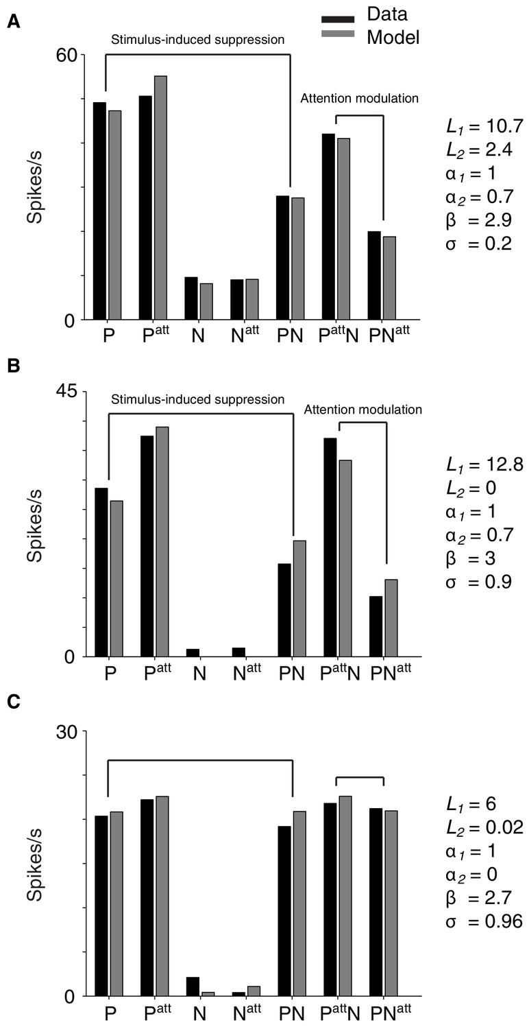
Example single-neuron responses and their corresponding model fits.
(A) Neuron with a preferred (P) and non-preferred (N) stimulus presented inside the cRF (cRF-cRF condition). Black: observed responses. Grey: modeled responses. P, Patt, N, Natt show the responses to the individually-presented preferred and non-preferred stimulus with attention away (P, N), or attention directed to the stimulus (Patt, Natt). PN shows the condition in which both stimuli were presented simultaneously with attention away (PN), attention directed toward the preferred stimulus (PattN), or directed toward the non-preferred stimulus (PNatt). The values of the model parameters for each example neuron are shown on the right. Note that these parameter values correspond to spike counts in a 250 ms window and should be multiplied by four to obtain spikes/s. This neuron's response is suppressed when a non-preferred stimulus is added to a preferred stimulus (P vs. PN). The model accounts for this difference because the non-preferred stimulus induces few excitation (small L2) but large enough suppression (α2). So suppression dominates over excitation. The model also captures the strong attention modulation (PattN vs. PNatt) through the β parameter, which multiplies the excitatory drive (L) and suppressive drive (α) of the attended stimulus. By increasing the weight of both drives, attention effectively focuses on the inputs related to the attended stimuli, as if the inputs from other stimuli were attenuated. So attention to a weak stimulus decreases the response, while attention to a strong stimulus increases the response (i.e. attention modulation). (B) Neuron with a cRF (P) and surround (N) stimulus (sRF-cRF condition). The model accounts for the observed suppression and attention modulation, which is similar to that of the neuron in A (cRF-cRF condition). (C) Neuron with a cRF (P) and surround (N) stimulus (sRF-cRF condition). The surround stimulus induces no surround suppression (low α2 and L2 value). As a result, shifting attention between the cRF and the surround stimulus leads to virtually no attention modulation.
Figure 6
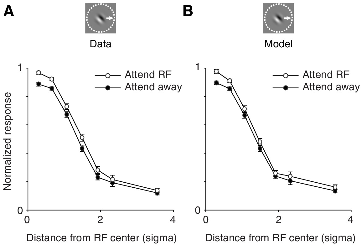
The spatially-tuned normalization model captures how attention modulates responses to single stimuli presented at various receptive field locations.
(A) Observed responses. Average response as a function of the distance between the single stimulus and the receptive field center, when the stimulus is attended (white) or unattended (black). (B) Same as (A) but for the modeled responses. The responses of each neuron were normalized to the maximum response across conditions in which a single stimulus was presented inside the receptive field. The receptive field distance is given by the Mahalanobis distance from the Gaussian receptive-field center. The Mahalanobis distance is akin to the number of standard deviations (σ) away from the receptive-field center. Only neurons whose receptive fields were well fitted with a two-dimensional Gaussian profile (>80% explained variance; 306 neurons; M1: 95; M2: 211) were included. Error bars represent ± SEM.
Figure 7
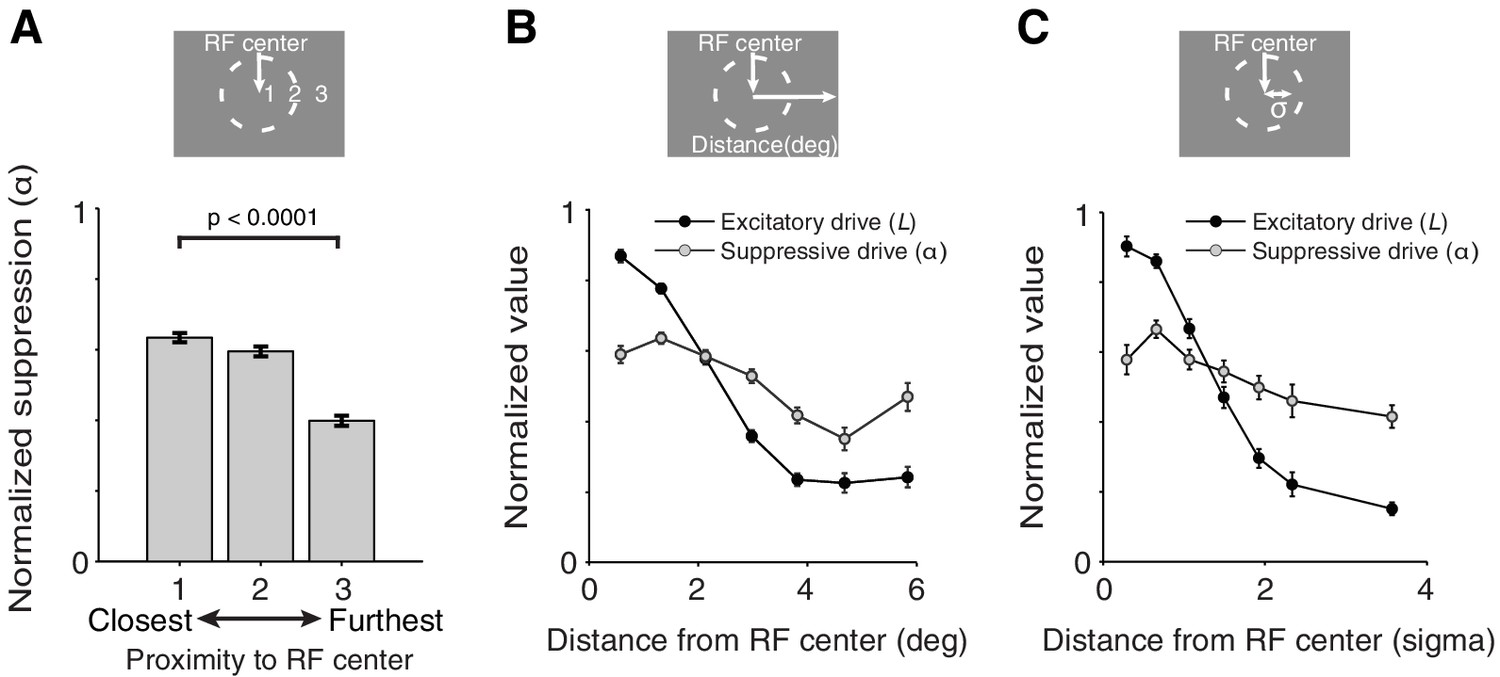
Spatially-tuned excitation and suppression decrease with distance from the receptive-field center, but at different rates.
(A) Each recording session we measured neuronal responses to stimuli presented at three different receptive-field locations (Figure 2A). The responses of each neuron were fitted with the spatially-tuned normalization model. The value of the suppression parameters α associated with each of the three measured receptive-field locations were ranked according to the proximity of those receptive-field locations to the neuron's receptive-field center: 1 being closest, and 3 being furthest away from the receptive-field center. The suppression parameter values were then normalized by the maximum α-value for each neuron. For each ranking number, the normalized suppression parameter values were subsequently averaged across neurons. Stimulus locations closest to the receptive-field center contributed more suppression to the neurons' response than those furthest away. (B) Average normalized suppressive drive (α, gray) and excitatory drive (L, black) as a function of the distance (in visual degrees) of its corresponding receptive-field location from the receptive-field center. The value of the excitatory drive parameter L for stimuli of different orientations were averaged per receptive-field location, and normalized by the maximum excitatory drive across the three measured receptive-field locations of a neuron. (C) Same as (B) but with an alternative distance measure, namely the Mahalanobis distance, which is akin to the number of standard deviations (σ) away from the receptive-field center. In (B) and (C), each excitatory-drive value L (black) has a corresponding suppressive-drive value α (gray). Error bars represent ± SEM.
Figure 8
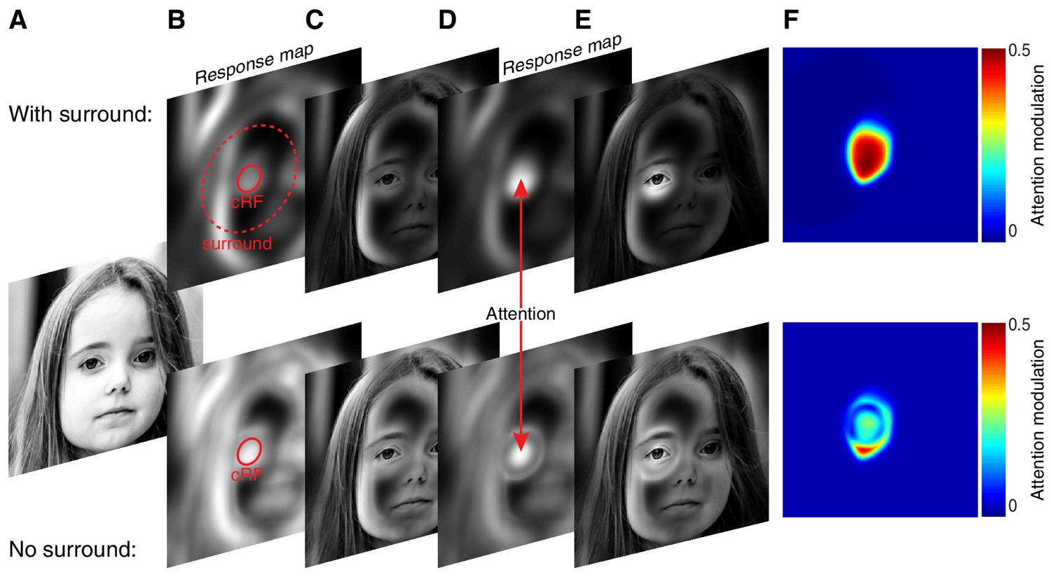
The surround may amplify spatial attention under natural viewing conditions.
(A) Original image. (B) Model neurons tiled the image. Each pixel contained one model neuron with its receptive-field centered on that pixel. An example cRFs (solid red) and surround (red dashed) for one neuron are shown. The radius of each neuron's surround was approximately five times larger than the radius of its cRF. The model neurons computed local contrast within the excitatory and suppressive component of their receptive field. The response maps show each neuron's response: neurons near high-contrast regions responded most as indicated by the luminance of the pixels. (C) Original image scaled according to the response map in (B). (D) Attention was directed to the left eye. Attention weighed the excitatory and suppressive inputs with its Gaussian kernel, resulting in stronger responses of the neurons with receptive fields near the attended location relative to neurons with receptive fields outside the locus of attention. (E) Original image scaled according to the response map in (D), illustrating the way attention changes the visual representation. (F) Attention modulation of each neuron, defined as (responseAtt - response) / (responseAtt + response). Here, response is the response map without attention as in (B), while responseAtt is the response map with attention as in (D). Upper panels (B–F) are based on model neurons with a suppressive surround. Lower panels (B–F) are based on model neurons without a suppressive surround, but with the same amount of suppression inside the cRF as the neurons with a suppressive surround.
Download links
A two-part list of links to download the article, or parts of the article, in various formats.
Downloads (link to download the article as PDF)
Open citations (links to open the citations from this article in various online reference manager services)
Cite this article (links to download the citations from this article in formats compatible with various reference manager tools)
Attention operates uniformly throughout the classical receptive field and the surround
eLife 5:e17256.
https://doi.org/10.7554/eLife.17256


