Figures and data in Mapping transiently formed and sparsely populated conformations on a complex energy landscape

Version of Record: October 4, 2016
Accepted Manuscript: August 23, 2016

Download
A two-part list of links to download the article, or parts of the article, in various formats.
Downloads (link to download the article as PDF)
- Article PDF
- Figures PDF
Open citations (links to open the citations from this article in various online reference manager services)
- Mendeley
Cite this article (links to download the citations from this article in formats compatible with various reference manager tools)
Yong Wang

Elena Papaleo

Kresten Lindorff-Larsen

(2016)
Mapping transiently formed and sparsely populated conformations on a complex energy landscape

eLife 5:e17505.

https://doi.org/10.7554/eLife.17505
- Download BibTeX
- Download .RIS
Cite
Share
CommentOpen annotations (there are currently 0 annotations on this page).

Figures
Videos
Tables

12 figures, 6 videos and 7 tables

Figures

Figure 1

Download asset Open asset

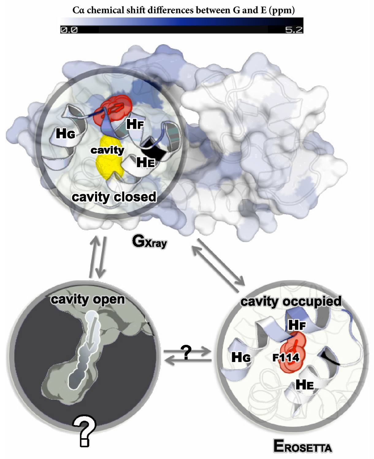
Structures of the major G and minor E states of L99A T4L and the hidden state hypothesis.

The X-ray structure of the G state ( $G_{X r a y}$ ; PDB ID code 3DMV) has a large internal cavity within the core of the C-terminal domain that is able to bind hydrophobic ligands. The structure of the E state …
https://doi.org/10.7554/eLife.17505.003

Figure 2 with 2 supplements

Download asset Open asset

Free energy landscape of the L99A variant of T4L.

In the upper panel, we show the projection of the free energy along $S_{p a t h}$ , representing the Boltzmann distribution of the force field employed along the reference path. Differently colored lines …
https://doi.org/10.7554/eLife.17505.004

Figure 2—figure supplement 1

Download asset Open asset

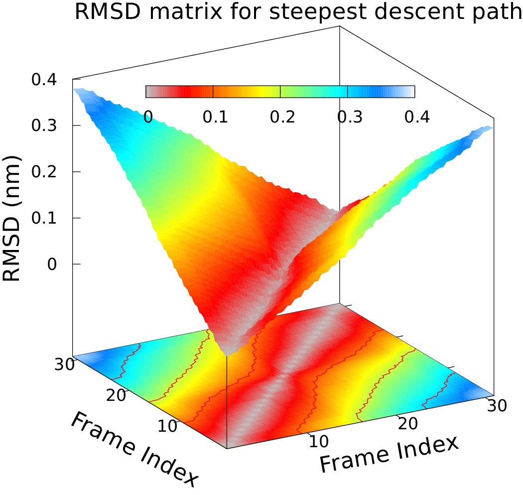
Approximately equidistant frames along the reference path.

The plot reveals a ‘gullwing’ shape of the matrix of pairwise RMSDs of the frames of the reference path, indicating that frames along the reference path are approximately equidistant. We used 31 …
https://doi.org/10.7554/eLife.17505.005

Figure 2—figure supplement 2

Download asset Open asset

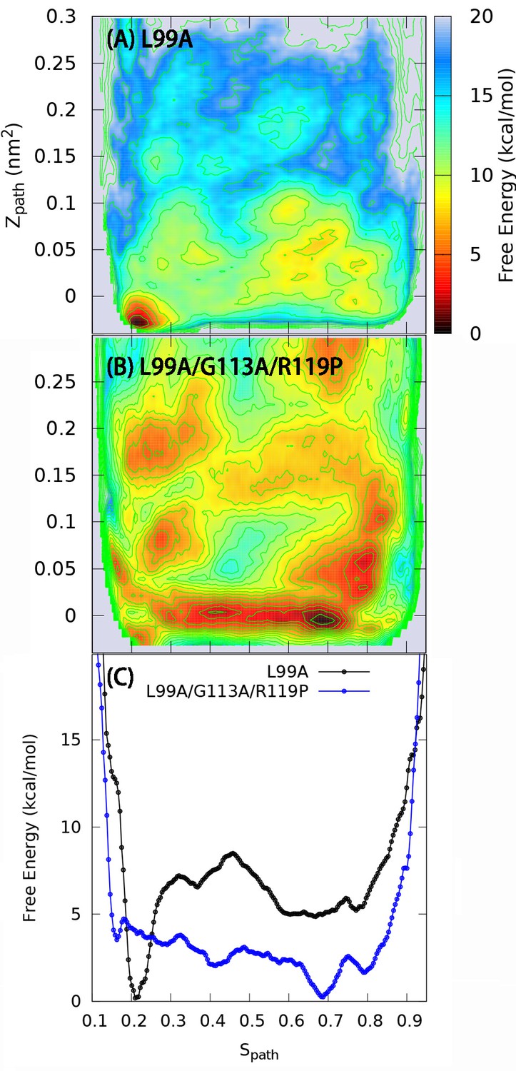
One and two dimensional free energy landscape of L99A and the triple mutant.

(A) The two-dimensional free energy surface F( $S_{p a t h}$ , $Z_{p a t h}$ ) of L99A sampled by a 667 ns PathMetaD simulation. (B) The two-dimensional free energy surface F( $S_{p a t h}$ , $Z_{p a t h}$ ) of the triple mutant sampled by a 961 ns …
https://doi.org/10.7554/eLife.17505.006

Figure 3

Download asset Open asset

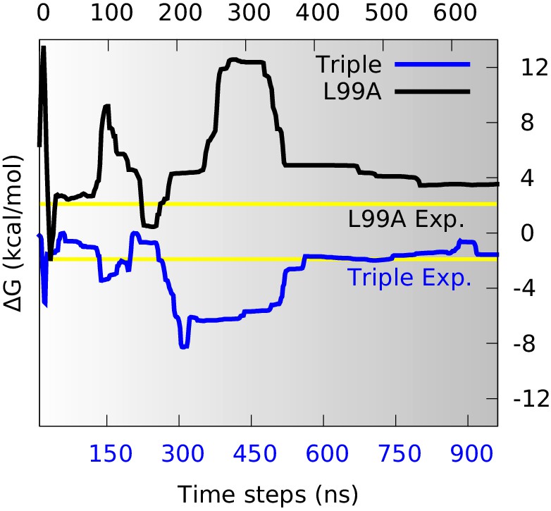
Estimation of free energy differences and comparison with experimental measurements.

We divided the global conformational space into two coarse-grained states by defining the separatrix at $S_{p a t h} = 0.46$ (0.48 for the triple mutant) in the free energy profile (Figure 2—figure supplement 2) …
https://doi.org/10.7554/eLife.17505.007

Figure 4 with 5 supplements

Download asset Open asset

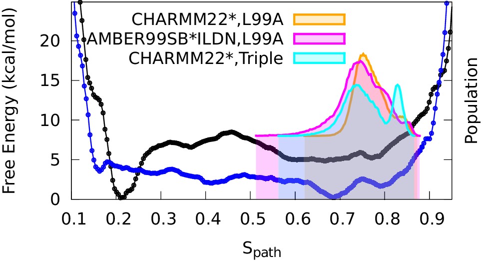
Conformational ensemble of the minor state as determined by CS biased, replica-averaged simulations.

We determined an ensemble of conformations corresponding to the E-state of L99A T4L using replica-averaged CSs as a bias term in our simulations. The distribution of conformations was projected onto …
https://doi.org/10.7554/eLife.17505.009

Figure 4—figure supplement 1

Download asset Open asset

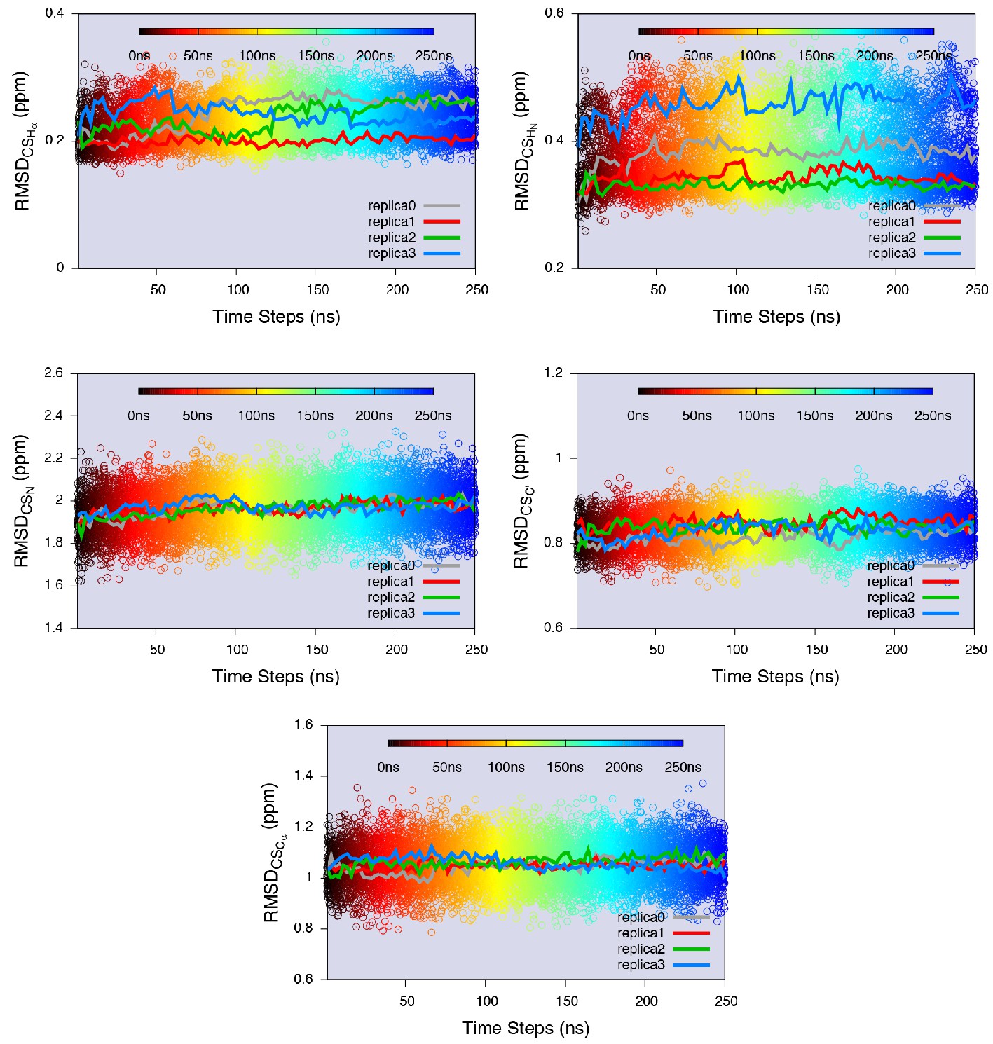
Equilibrium sampling of conformational regions of the E state of L99A by CS-restrained replica-averaged simulation.

We calculated the RMSD between the experimental CSs and the values back-calculated by CamShift (Kohlhoff et al., 2009) as implemented in ALMOST (Fu et al., 2014). We projected a 250 ns MD trajectory …
https://doi.org/10.7554/eLife.17505.010

Figure 4—figure supplement 2

Download asset Open asset

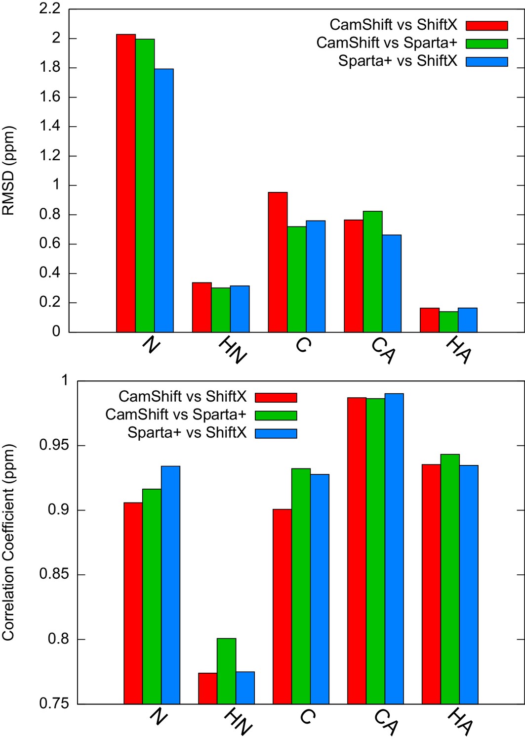
Estimation of the inherent uncertainty of the chemical shift calculation by different algorithms: CamShift (Kohlhoff et al., 2009), ShiftX (Neal et al., 2003) and Sparta+ (Shen and Bax, 2010).

Using $E_{R O S E T T A}$ as the reference structure, we calculated the chemical shifts using different algorithms and compared the correlation coefficients and RMSD between them.

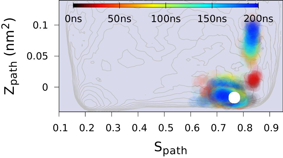
https://doi.org/10.7554/eLife.17505.011

Figure 4—figure supplement 3

Download asset Open asset

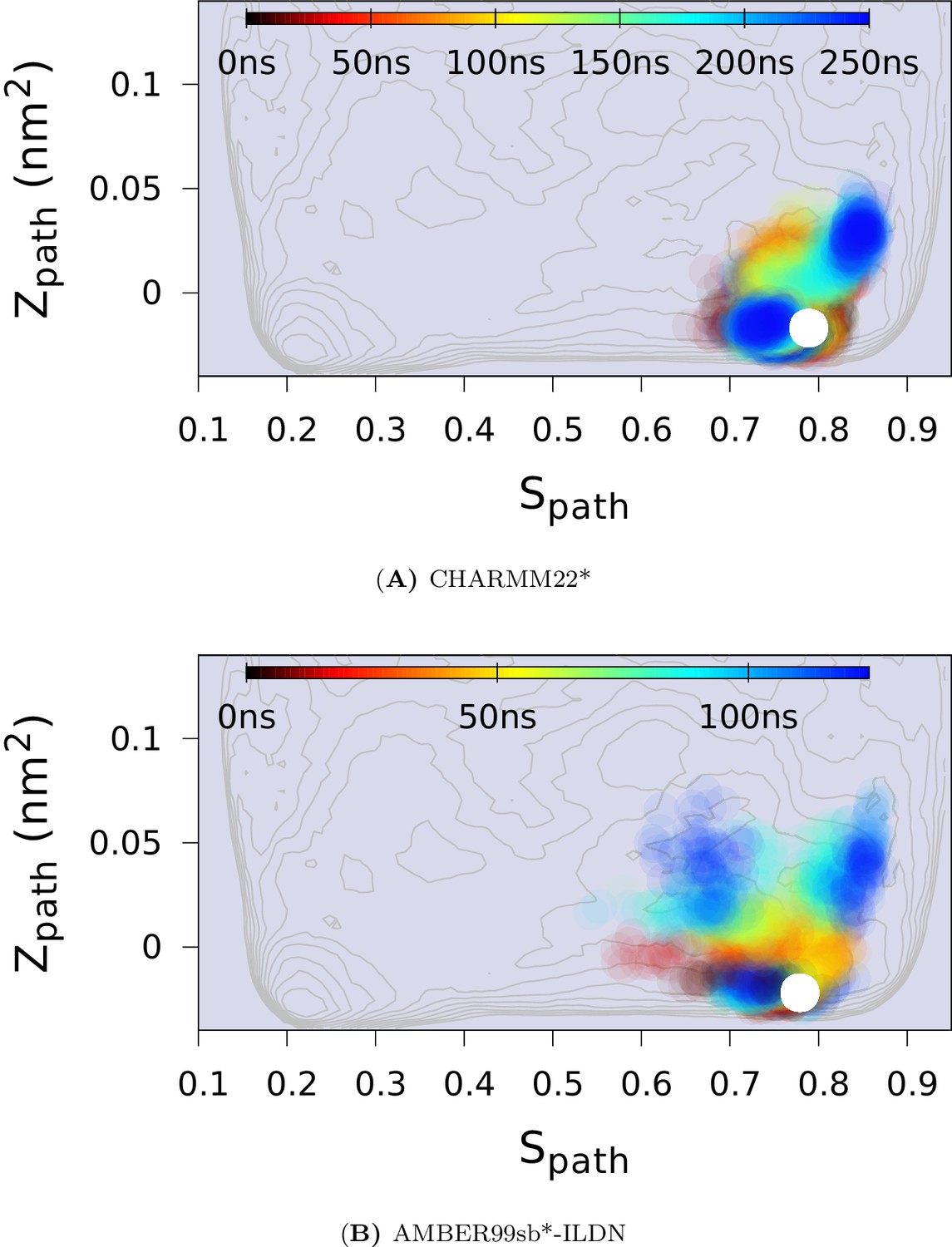
Force field dependency of the replica averaged MD simulations of L99A with chemical shift restraints.

The chemical shifts of the E state of L99A (BMRB 17604) were used. (A) The simulation with CHARMM22* force field. (B) The simulation with Amber ff99SB*-ILDN force field.

https://doi.org/10.7554/eLife.17505.012

Figure 4—figure supplement 4

Download asset Open asset

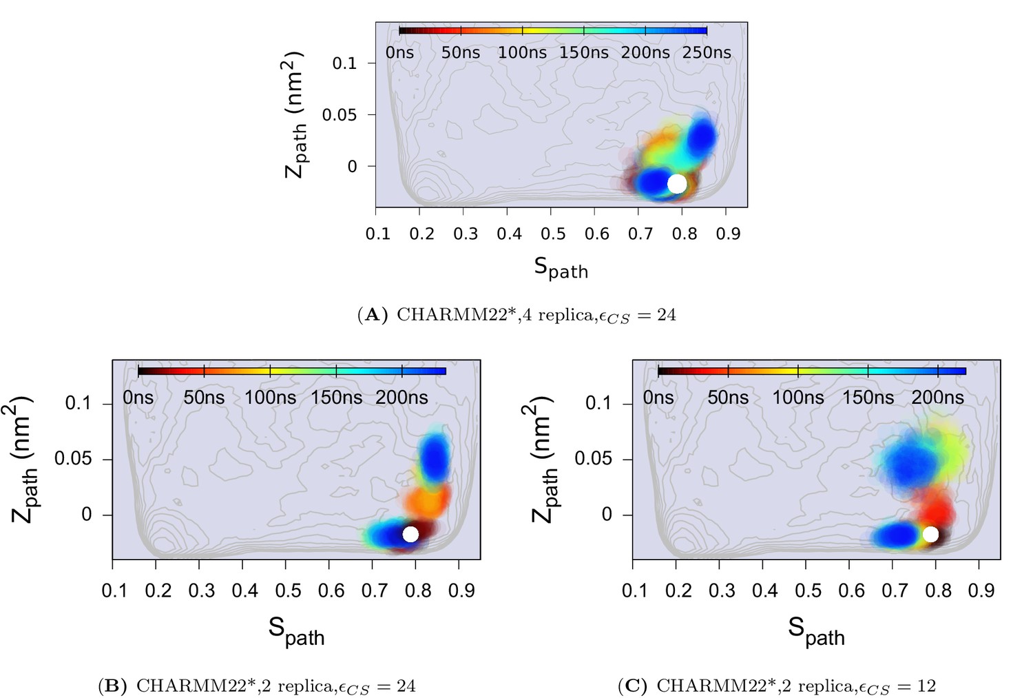
Effect of changing the force constant and number of replicas in CS-restrained simulation of L99A.

(A) N = 4, $ϵ_{C S} = 24$ KJ · mol⁻¹. (B) N = 2, $ϵ_{C S} = 24$ KJ · mol⁻¹. (C) N = 2, $ϵ_{C S} = 12$ KJ · mol⁻¹. N refers to the number of replicas that the CS values are averaged over. The CHARMM22* force field was used in these …
https://doi.org/10.7554/eLife.17505.013

Figure 4—figure supplement 5

Download asset Open asset

Replica-averaged CS-restrained MD simulation of a T4L triple mutant (L99A/G113A/R119P).

Chemical shift restraints were from BMRB 17,603 and CHARMM22* force field was used.

https://doi.org/10.7554/eLife.17505.014

Figure 5 with 3 supplements

Download asset Open asset

Mechanisms of the G-E conformational exchanges explored by reconnaissance metadynamics.

Trajectories labeled as Trj1 (magenta), Trj2 (blue) and Trj3 (green and orange) are from the simulations RUN10, RUN11 and RUN12 (Appendix 1—table 1), respectively. There are multiple routes …
https://doi.org/10.7554/eLife.17505.015

Figure 5—figure supplement 1

Download asset Open asset

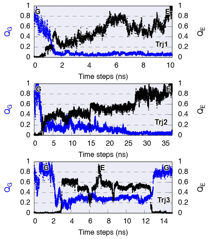
Complete G-to-E transitions of L99A obtained by reconnaissance metadynamics simulations.

The state-specific fraction of contacts (Wang et al., 2012), and , were employed to monitor the conformational transitions to G and E state, respectively. Trajectories Trj1, Trj2 and Trj3 are from …
https://doi.org/10.7554/eLife.17505.016

Figure 5—figure supplement 2

Download asset Open asset

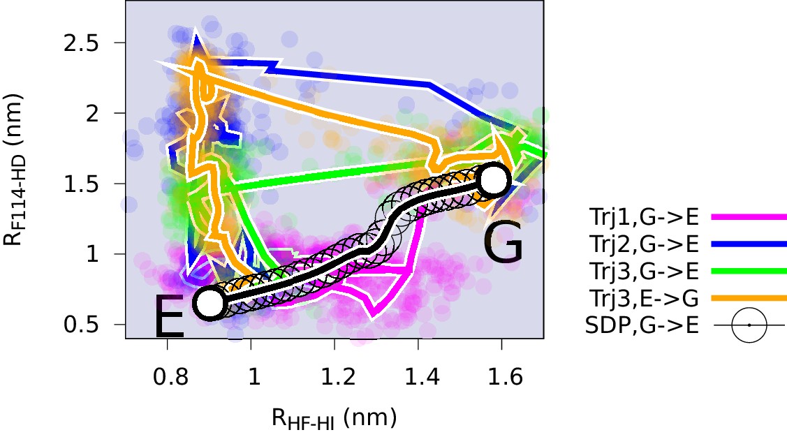
Conformational transitions between the G and E states monitored by other order parameters.

Trajectories Trj1 (magenta), Trj2 (blue) and Trj3 (green and orange) are from the simulations RUN10, RUN11 and RUN12 (Appendix 1—table 2), respectively. The steepest descent path (SDP, black) used …
https://doi.org/10.7554/eLife.17505.017

Figure 5—figure supplement 3

Download asset Open asset

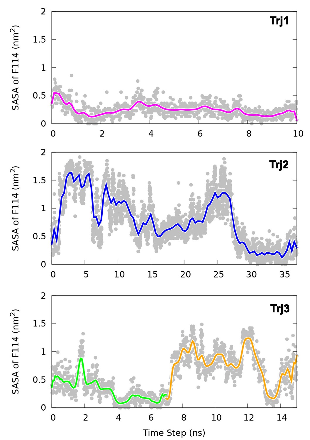
Solvent accessible surface area (SASA) calculation of the side chain of F114.

The figure suggests in the direct $G ⇋ E$ transitions (Trj1 and first half of Trj3) F114 can rotate its side chain inside the protein core. In contrast, in the $G ⇋ I_{0.36} ⇋ E$ route (Trj2 and second half of Trj3) the …
https://doi.org/10.7554/eLife.17505.018

Figure 6 with 4 supplements

Download asset Open asset

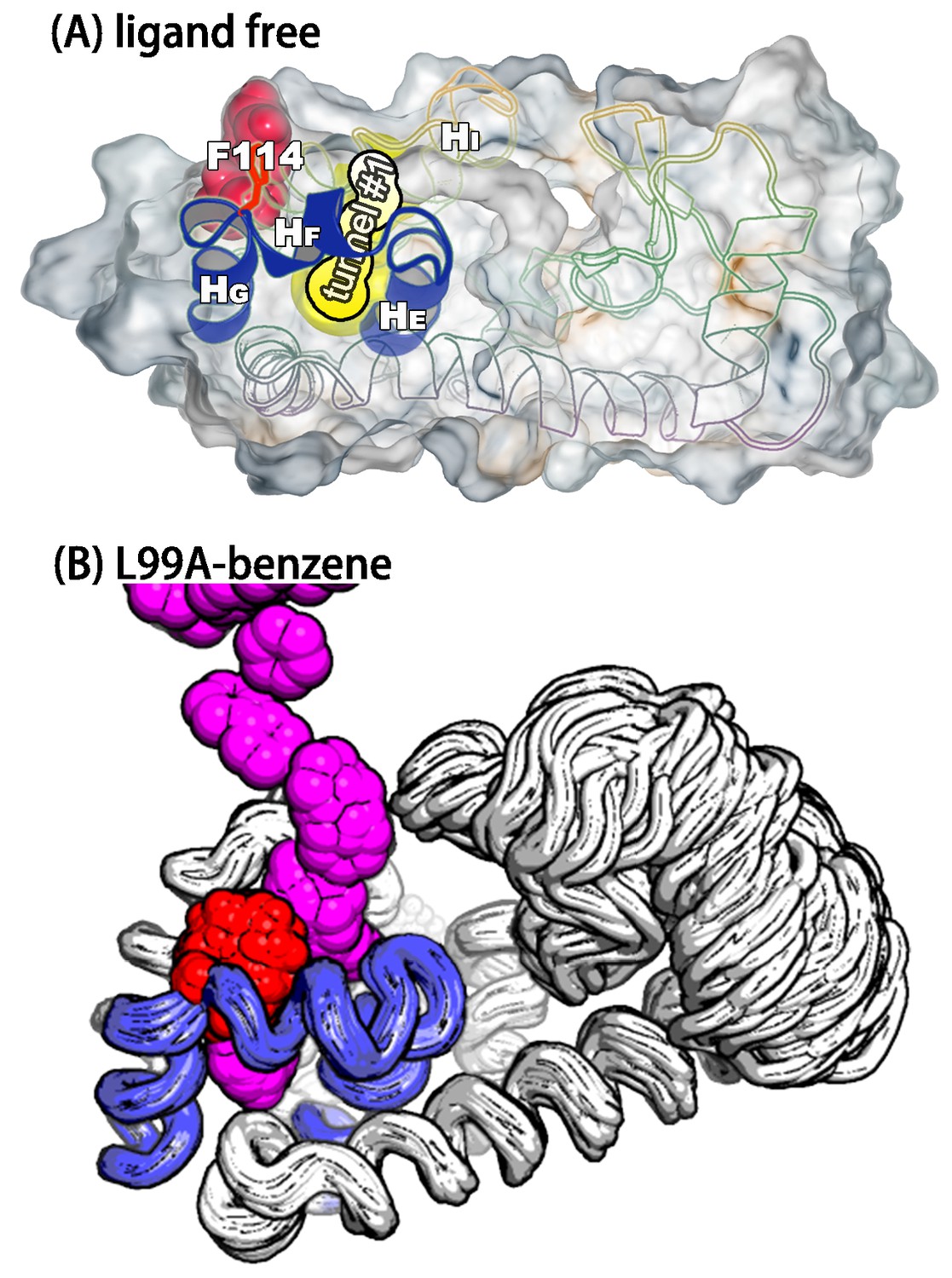
A transiently formed tunnel from the solvent to the cavity is a potential ligand binding pathway.

(A) We here highlight the most populated tunnel structure (tunnel $# 1$ ), that has an entrance located at the groove between helix F ( $H_{F}$ ) and helix I ( $H_{I}$ ). Helices E, F and G (blue) and F114 (red) are …
https://doi.org/10.7554/eLife.17505.024

Figure 6—figure supplement 1

Download asset Open asset

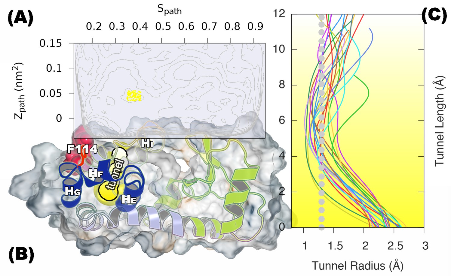
A transiently formed tunnel from the solvent to the cavity forms in the $I_{0.36}$ state.

(A) Typical structures from the $I_{0.36}$ state sampled in the simulation (between 430 ns and 447 ns) are mapped onto the free energy surface, and represented by yellow points. (B) The cavity-related …
https://doi.org/10.7554/eLife.17505.025

Figure 6—figure supplement 2

Download asset Open asset

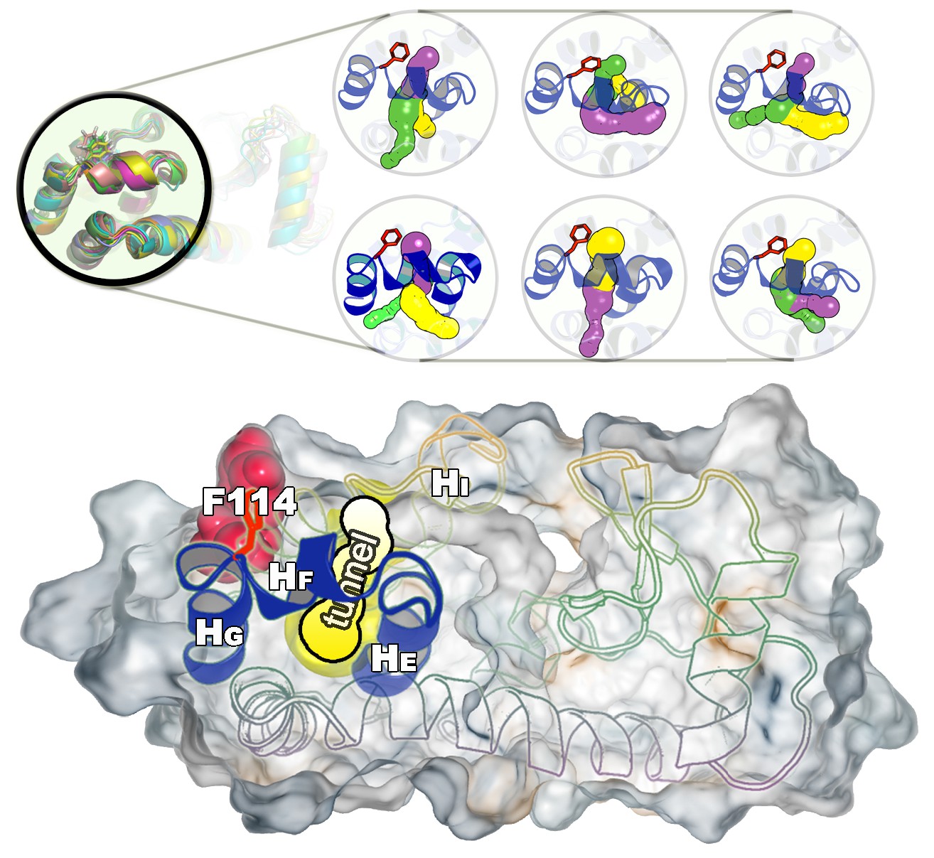
Representative structures of the cavity region in the $I_{0.36}$ state.

The figure shows six representative structures of the cavity region revealing multiple tunnels that connect the cavity with the protein surface. The different colours correspond to different tunnels …
https://doi.org/10.7554/eLife.17505.026

Figure 6—figure supplement 3

Download asset Open asset

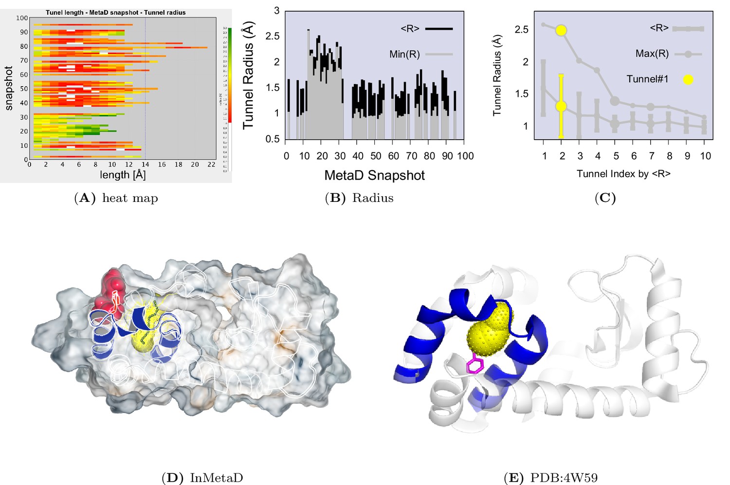
Tunnel clustering analysis on $I_{0.36}$ state.

The clustering of tunnels was performed using the CAVER Analyst software (Kozlikova et al., 2014) and the average-link hierarchical algorithm based on the calculated matrix of pairwise tunnel …
https://doi.org/10.7554/eLife.17505.027

Figure 6—figure supplement 4

Download asset Open asset

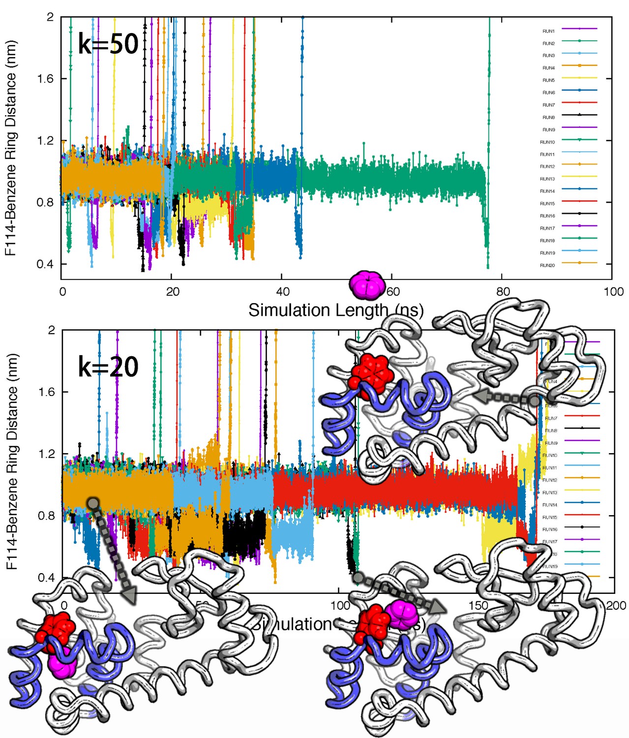
Ligand unbinding pathways revealed by ABMD simulations.

The figure shows how ABMD simulations allow us to observe the ligand benzene escape from the internal binding site. We performed two sets of 20 simulations using two different force constants for …
https://doi.org/10.7554/eLife.17505.028

Appendix 1—figure 1

Download asset Open asset

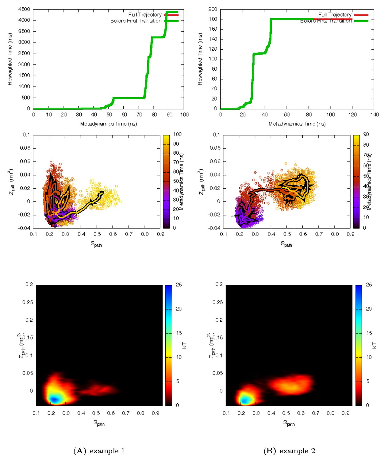
Two representative InMetaD trajectories of L99A with G to E transitions.

The time point, t′, for the first transition from G to E is identified when the system evolves into conformational region of S_path > 0.55 and Z_path < 0.01. We then calculate the unbiased passage …
https://doi.org/10.7554/eLife.17505.030

Appendix 1—figure 2

Download asset Open asset

Two representive InMetaD trajectories of L99A with E to G transitions of L99A.

First transition time for G to E transition is identified when the system evolves into conformational region of S_path < 0.28 and Z_path < −0.01.

https://doi.org/10.7554/eLife.17505.031

Appendix 1—figure 3

Download asset Open asset

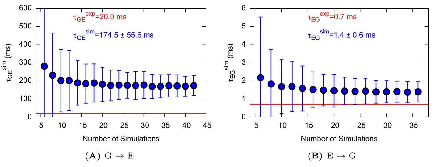
Characteristic transition times between G and E states of L99A.

The error bars represent the standard deviation of τ obtained from a bootstrap analysis.

https://doi.org/10.7554/eLife.17505.032

Appendix 1—figure 4

Download asset Open asset

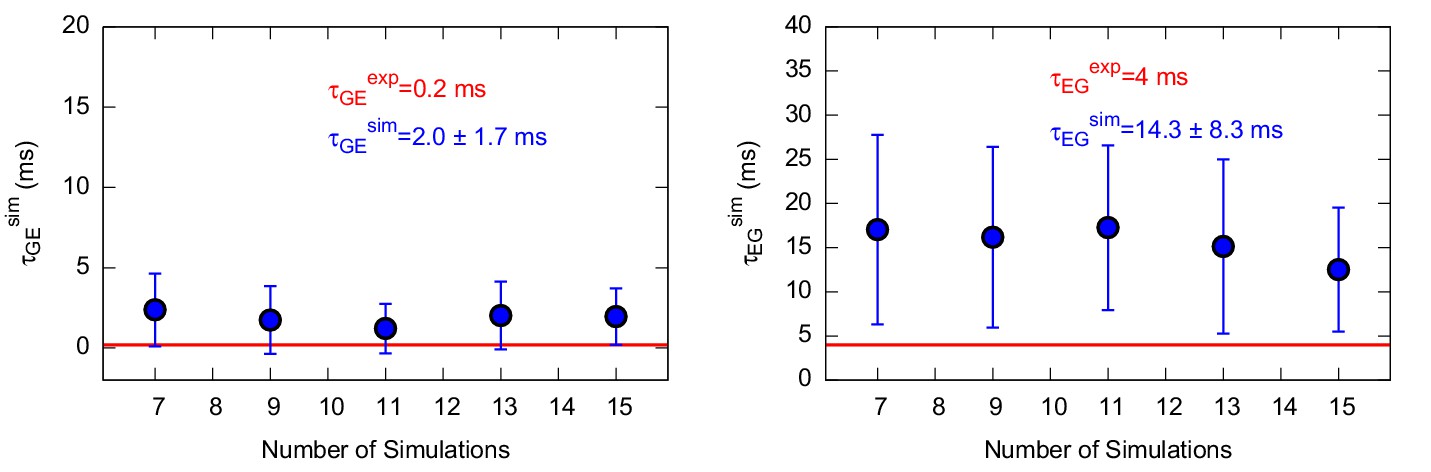
Characteristic transition times between G and E states of the triple mutant.

The figure shows the characteristic transition time τ_G→E (left panel) and τ_E→G (right panel) of the triple mutant as a function of the size of a subsample of transition times randomly extracted from …
https://doi.org/10.7554/eLife.17505.033

Appendix 1—figure 5

Download asset Open asset

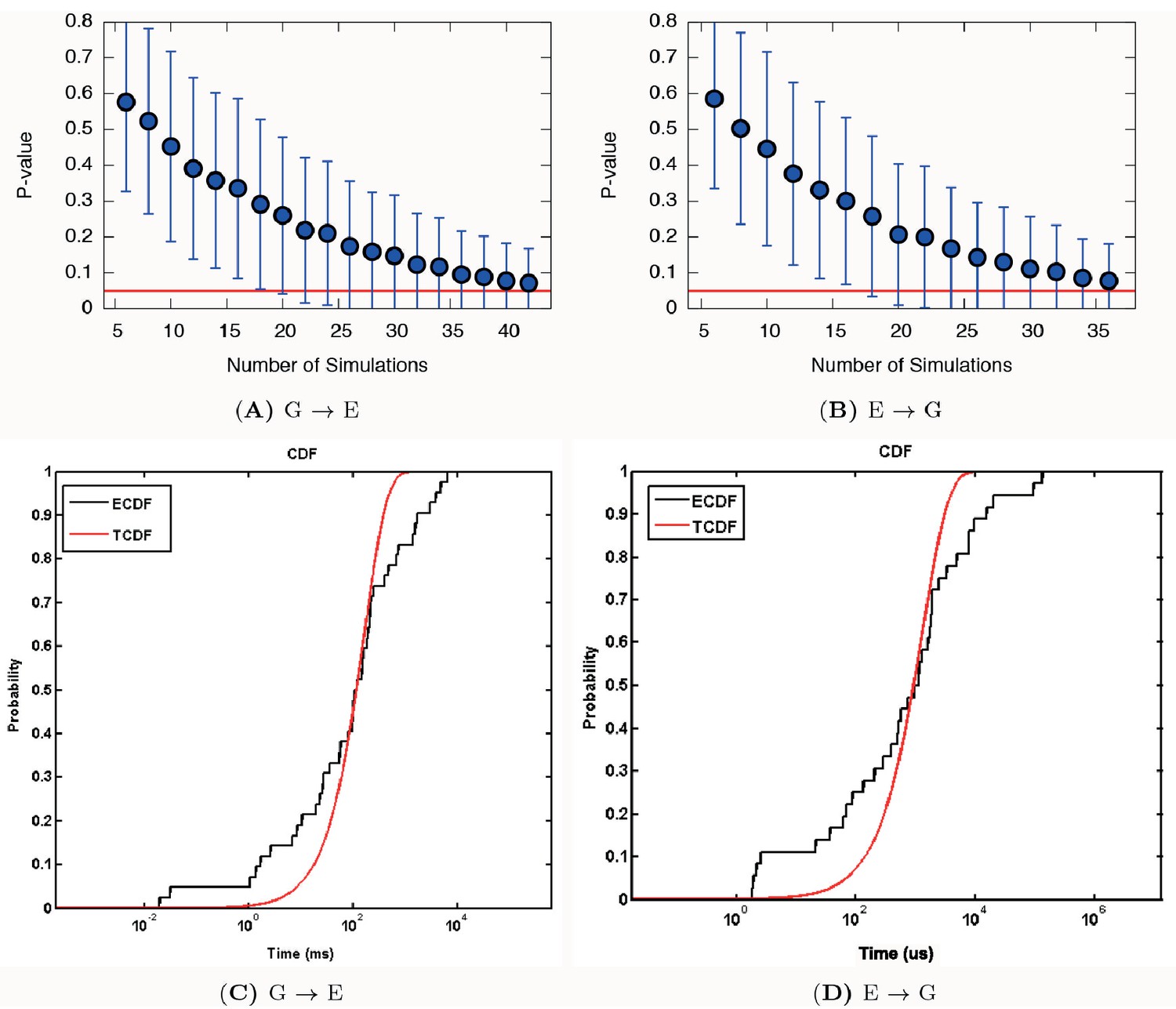
Poisson fit analysis for G to E transitions and E to G transitions of L99A.

We show the ECDF (the empirical cumulative distribution function) and TCDF (the theoretical cumulative distribution function) in black and blue lines, respectively. The respective p-values are …
https://doi.org/10.7554/eLife.17505.034

Appendix 1—figure 6

Download asset Open asset

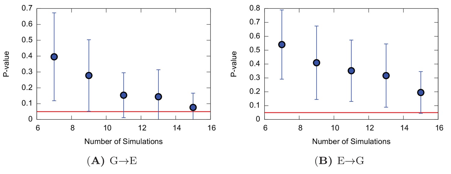
Poisson fit analysis for G to E transitions and E to G transitions of the triple mutant.

The figure shows the p-values of the Poisson fit analysis of G → E (A) and E → G (B) transition times as a function of the size of a subsample of transition times randomly extracted from the main …
https://doi.org/10.7554/eLife.17505.035

Videos

Video 1

Download asset

posterframe for video — Trajectory of the G-to-E conformational transition observed in Trj1, corresponding to the red trajectory in Figure 5.

The backbone of L99A is represented by white ribbons, Helices E, F and G are highlighted in blue, while F114 is represented by red spheres.

https://doi.org/10.7554/eLife.17505.019

Video 2

Download asset

Video 3

Download asset

Video 4

Download asset

Video 5

Download asset

Video 6

Download asset

Tables

Table 1

Free energy differences and rates of conformational exchange.

https://doi.org/10.7554/eLife.17505.008

	$τ_{G \to E}$ (ms)	$τ_{E \to G}$ (ms)	$Δ G$ (kcal mol⁻¹)
L99A
NMR	20	0.7	2.1
InMetaD	175 $\pm$ 56	1.4 $\pm$ 0.6	2.9 $\pm$ 0.5
PathMetaD			3.5
L99A/G113A/R119P
NMR	0.2	4	-1.9
InMetaD	2.0 $\pm$ 1.7	14.3 $\pm$ 8.3	-1.2 $\pm$ 1.1
PathMetaD			-1.6

Appendix 1—table 1

Simulation details.

https://doi.org/10.7554/eLife.17505.036

Method	label	system	init	length	force field	CVs	parameters	T (K)	software version
PathMetaD	RUN1	L99A	G	667 ns	CHARMM22*	$S_{p a t h}$ , $Z_{p a t h}$	$γ$ =20^†, $τ_{D}$ =1 ps^‡, $τ_{G}$ =1 ps^§, $ω_{0}$ =1.5^¶	298	PLUMED2.1, GMX4.6
PathMetaD	RUN2	L99A, G113A, R119P	G	961 ns	CHARMM22*	$S_{p a t h}$ , $Z_{p a t h}$	$γ$ =20, $τ_{D}$ =1 ps, $τ_{G}$ =1ps, $ω_{0}$ =1.5	298	PLUMED2.1, GMX5.0
CS-restrained MD	RUN3	L99A	E	252 ns	CHARMM22*		N^#=4, $ϵ_{C S} = 24$ **	298	PLUMED2.1, ALMOST2.1, GMX5
CS-restrained MD	RUN4	L99A	E	233 ns	CHARMM22*		N=2, $ϵ_{C S} = 24$	298	PLUMED2.1, ALMOST2.1, GMX5
CS-restrained MD	RUN5	L99A	E	221 ns	CHARMM22*		N=2, $ϵ_{C S} = 12$	298	PLUMED2.1, ALMOST2.1, GMX5
CS-restrained MD	RUN6	L99A	E	125 ns	AMBER99sb*ILDN		N=4, $ϵ_{C S} = 24$	298	PLUMED2.1, ALMOST2.1, GMX5
CS-restrained MD	RUN7	L99A	E	190 ns	AMBER99sb*ILDN		N=2, $ϵ_{C S} = 12$	298	PLUMED2.1, ALMOST2.1, GMX5
CS-restrained MD	RUN8	L99A, G113A, R119P	G	204 ns	CHARMM22*		N=4, $ϵ_{C S} = 24$	298	PLUMED2.1, ALMOST2.1, GMX5
CS-restrained MD	RUN9	L99A, G113A, R119P	G	200 ns	CHARMM22*		N=2, $ϵ_{C S} = 24$	298	PLUMED2.1, ALMOST2.1, GMX5
Reconnaissance MetaD	RUN10	L99A	G	120 ns	CHARMM22*	2,3,4,5	$Δ T$ =10000^††, $Δ t$ =250	298	PLUMED1.3, GMX4.5
Reconnaissance MetaD	RUN11	L99A	G	85 ns	CHARMM22*	2,3,4,5	10000, 250	298	PLUMED1.3, GMX4.5
Reconnaissance MetaD	RUN12	L99A	G	41 ns	CHARMM22*	2,3,4,5,7,8	100000, 500	298	PLUMED1.3, GMX4.5
PT-WT-MetaD	RUN13	L99A	G	961 ns	CHARMM22*	1,2,3,7,8	$γ$ =20, $ω_{0}$ =0.5	297 298^‡‡ 303 308 316 325 341 350 362	PLUMED 1.3, GMX4.5
PT-WT-MetaD	RUN14	L99A	G	404 ns	CHARMM22*	1,2,3,6,7	$γ$ =20, $ω_{0}$ =0.5	297 298 303 308 316 325 333 341 350	PLUMED 1.3, GMX4.5
PT-WT-MetaD	RUN15	L99A	G	201 ns	CHARMM22*	1,2,3,6	$γ$ =20, $ω_{0}$ =0.5	297 298 303 308 316 325 333 341 350	PLUMED 1.3, GMX4.5
PT-WT-MetaD	RUN16	L99A	G	511 ns	CHARMM22*	1,2,3,4,5	$γ$ =5, $ω_{0}$ =0.5	295 298 310 325 341 358 376	PLUMED 1.3, GMX4.5
PT-WT-MetaD	RUN17	L99A	G	383 ns	CHARMM22*	1,2,3,4,5	$γ$ =20, $ω_{0}$ =0.5	298 305 313 322 332 337 343	PLUMED 1.3, GMX4.5
PT-WT-MetaD	RUN18	L99A	E	365 ns	CHARMM22*	1	$γ$ =20, $ω_{0}$ =0.5	298 302 306 311 317 323 330 338	PLUMED 1.3, GMX4.5
plain MD	RUN19	L99A	G	400 ns	CHARMM22*			298	GMX5.0
plain MD	RUN20	L99A	E	400 ns	CHARMM22*			298	GMX5.0
plain MD	RUN21	L99A	G	400 ns	AMBER99sb*ILDN			298	GMX5.0
plain MD	RUN22	L99A	E	400 ns	AMBER99sb*ILDN			298	GMX5.0
plain MD	RUN23	L99A,G113A,R119P	G	400 ns	CHARMM22*			298	GMX5.0
plain MD	RUN24	L99A,G113A,R119P	E	400 ns	CHARMM22*			298	GMX5.0
plain MD	RUN25	L99A,G113A,R119P	G	400 ns	AMBER99sb*ILDN			298	GMX5.0
plain MD	RUN26	L99A,G113A,R119P	E	400 ns	AMBER99sb*ILDN			298	GMX5.0
InMetaD	RUN27-68^§§	L99A	G		CHARMM22*	$S_{p a t h}$ , $Z_{p a t h}$	$γ$ =20, $τ_{G}$ =80 ps, $ω_{0}$ =1.0, $σ_{S}$ =0.016^¶¶, $σ_{Z}$ =0.002^##	298	PLUMED2.1, GMX5
InMetaD	RUN69-104***	L99A	E		CHARMM22*	$S_{p a t h}$ , $Z_{p a t h}$	$γ$ =20, $τ_{G}$ =80 ps, $ω_{0}$ =1.0, $σ_{S}$ =0.016, $σ_{Z}$ =0.002	298	PLUMED2.1, GMX5
InMetaD	RUN105-119	L99A,G113A,R119P	G		CHARMM22*	$S_{p a t h}$ , $Z_{p a t h}$	$γ$ =15, $τ_{G}$ =100ps, $ω_{0}$ =0.8, $σ_{S}$ =0.016^¶¶, $σ_{Z}$ =0.002^##	298	PLUMED2.2, GMX5.1.2
InMetaD	RUN120-134	L99A,G113A,R119P	E		CHARMM22*	$S_{p a t h}$ , $Z_{p a t h}$	$γ$ =15, $τ_{G}$ =100 ps, $ω_{0}$ =0.8, $σ_{S}$ =0.016^¶¶, $σ_{Z}$ =0.002^##	298	PLUMED2.2, GMX5.1.2
ABMD	RUN135-154	L99A-Benzene	bound		CHARMM22*	$R M S D_{b e n z e n e}$	K=50 KJ · mol⁻¹ · nm⁻², $S_{t a r g e t} = 4.0$ nm	298	PLUMED2.2, GMX5.1.2
ABMD	RUN155-174	L99A-Benzene	bound		CHARMM22*	$R M S D_{b e n z e n e}$	K=20 KJ · mol⁻¹ · nm⁻², $S_{t a r g e t} = 4.0$ nm	298	PLUMED2.2, GMX5.1.2

^† $γ$ is the bias factor.
^‡ $τ_{D}$ is the characteristic decay time used for the dynamically-adapted Gaussian potential.
^§ $τ_{G}$ is the deposition frequency of Gaussian potential.
^¶ $ω_{0}$ is the height of the deposited Gaussian potential (in KJ · mol⁻¹).
^# N is the number of replicas.
** $ϵ_{C S}$ is the strength of chemical shift restraints (in KJ · mol⁻¹ · ppm⁻²).
^†† $Δ T$ means RUN_FREQ and $Δ t$ means STORE_FREQ. Other parameters: BASIN_TOL=0.2, EXPAND_PARAM=0.3, INITIAL_SIZE=3.0.
^‡‡ Replica at 298 K is the neutral replica without energy bias.
^§§42 trajectories collected for G-to-E transitions.
^¶¶ $σ_{S}$ is the Gaussian width of $S_{p a t h}$ .
^## $σ_{Z}$ is the Gaussian width of $Z_{p a t h}$ (in nm²).
***36 trajectories collected for E-to-G transitions.

Appendix 1—table 2

Definition of collective variables.

https://doi.org/10.7554/eLife.17505.037

CV	definitions	parameters	purpose
1	total energy	bin=500	enhance energy fluctuations
2	dihedral angle of $C_{α}$ atoms of consecutive residues F104-Q105-M106-G107	$σ$ =0.1
3	dihedral angle of $C_{α}$ atoms of consecutive residues G113-F114-T115-N116	$σ$ =0.1
4	$Q_{G}$ , distance in contact map space to the $G_{X r a y}$ structure	$σ$ =0.5
5	$Q_{E}$ , distance in contact map space to the $E_{R O S E T T A}$ structure	$σ$ =0.5
6	distance between $Q_{G}$ and $Q_{E}$	$σ$ =0.5
7	number of backbone hydrogen bonds formed between M102 and G107	$σ$ =0.1
8	dihedral correlation between the $C_{α}$ dihedral angles of consecutive residues in segment N101-G107	$σ$ =0.1
9	global RMSD to the whole protein	wall potential	avoid sampling unfolding space

Appendix 1—table 3

Average root-mean-square deviation ( $< R M S D >$ in units of ppm) between experimental CSs and those from the CS-restrained replica-averaged simulations.

https://doi.org/10.7554/eLife.17505.038

Nucleus	RUN3	RUN4	RUN5	RUN6	RUN7	RUN8	RUN9
$C^{'}$	0.833	0.655	0.776	0.854	0.793	0.907	0.727
$C_{α}$	1.055	0.879	0.929	1.065	0.940	1.103	0.894
$N$	1.966	1.707	1.771	1.967	1.780	2.011	1.828
$H_{N}$	0.379	0.275	0.291	0.368	0.284	0.414	0.286
$H_{A}$	0.232	0.183	0.186	0.242	0.182	0.246	0.183

Appendix 1—table 4

Parameter set used in tunnel analysis using CAVER3.0 (Chovancova et al., 2012) and CAVER Analyst1.0 (Kozlikova et al., 2014).

https://doi.org/10.7554/eLife.17505.039

Minimum probe radius	0.9 Å
Shell depth	4
Shell radius	3
Clustering threshold	3.5
Starting point optimization
Maximum distance	3 Å
Desired radius	5 Å

Appendix 1—table 5

Clustering analysis of tunnels (top three listed).

https://doi.org/10.7554/eLife.17505.040

Index	Population	Maximal bottleneck radius (Å)	Average bottleneck radius (Å)
#1	27%	2.5	1.3
#2	20%	1.4	1.0
#3	15%	1.3	1.0

Appendix 1—table 6

Unbinding Pathways Explored by ABMD ( $R M S D_{B N Z}$ as CV).

https://doi.org/10.7554/eLife.17505.041

	k=20 kJ/(mol · nm⁻²)		k=50 kJ/(mol · nm⁻²)
Index	Length	Path	Length	Path
RUN1	56 ns	P1	27 ns	P2
RUN2	36 ns	P2	78 ns	P1
RUN3	43 ns	P1	6 ns	P1
RUN4	43 ns	P1	35 ns	P1
RUN5	77 ns	P2	10 ns	P1
RUN6	176 ns	P1	44 ns	P1
RUN7	41 ns	P1	18 ns	P1
RUN8	106 ns	P1	15 ns	P1
RUN9	72 ns	P1	7 ns	P1
RUN10	107 ns	P1	2 ns	P1
RUN11	61 ns	P1	20 ns	P2
RUN12	58 ns	P2	26 ns	P1
RUN13	64 ns	P1	31 ns	P2
RUN14	173 ns	P2	20 ns	P1
RUN15	172 ns	P1	34 ns	P1
RUN16	74 ns	P2	22 ns	P1
RUN17	20 ns	P1	17 ns	P1
RUN18	34 ns	P1	35 ns	P2
RUN19	91 ns	P1	21 ns	P2
RUN20	61 ns	P1	18 ns	P1
Cost	1.6 μs		0.5 μs
Summary
P1	75% (15/20)		75% (15/20)
P2	25% (5/20)		25% (5/20)

Downloads (link to download the article as PDF)

Open citations (links to open the citations from this article in various online reference manager services)

Cite this article (links to download the citations from this article in formats compatible with various reference manager tools)

Figures

Structures of the major G and minor E states of L99A T4L and the hidden state hypothesis.

Free energy landscape of the L99A variant of T4L.

Approximately equidistant frames along the reference path.

One and two dimensional free energy landscape of L99A and the triple mutant.

Estimation of free energy differences and comparison with experimental measurements.

Conformational ensemble of the minor state as determined by CS biased, replica-averaged simulations.

Equilibrium sampling of conformational regions of the E state of L99A by CS-restrained replica-averaged simulation.

Estimation of the inherent uncertainty of the chemical shift calculation by different algorithms: CamShift (Kohlhoff et al., 2009), ShiftX (Neal et al., 2003) and Sparta+ (Shen and Bax, 2010).

Force field dependency of the replica averaged MD simulations of L99A with chemical shift restraints.

Effect of changing the force constant and number of replicas in CS-restrained simulation of L99A.

Replica-averaged CS-restrained MD simulation of a T4L triple mutant (L99A/G113A/R119P).

Mechanisms of the G-E conformational exchanges explored by reconnaissance metadynamics.

Complete G-to-E transitions of L99A obtained by reconnaissance metadynamics simulations.

Conformational transitions between the G and E states monitored by other order parameters.

Solvent accessible surface area (SASA) calculation of the side chain of F114.

A transiently formed tunnel from the solvent to the cavity is a potential ligand binding pathway.

A transiently formed tunnel from the solvent to the cavity forms in the $I_{0.36}$ state.

Representative structures of the cavity region in the $I_{0.36}$ state.

Tunnel clustering analysis on $I_{0.36}$ state.

Ligand unbinding pathways revealed by ABMD simulations.

Two representative InMetaD trajectories of L99A with G to E transitions.

Two representive InMetaD trajectories of L99A with E to G transitions of L99A.

Characteristic transition times between G and E states of L99A.

Characteristic transition times between G and E states of the triple mutant.

Poisson fit analysis for G to E transitions and E to G transitions of L99A.

Poisson fit analysis for G to E transitions and E to G transitions of the triple mutant.

Videos

Trajectory of the G-to-E conformational transition observed in Trj1, corresponding to the red trajectory in Figure 5.

Trajectory of the G-to-E conformational transition observed in Trj2, corresponding to the blue trajectory in Figure 5.

Trajectory of the G-to-E conformational transition observed in Trj3, corresponding to the green trajectory in Figure 5.

Trajectory of the E-to-G conformational transition observed in Trj3, corresponding to the yellow trajectory in Figure 5.

Movie of the calculated two-dimensional free energy landscape of L99A as a function of simulation time.

A typical trajectory of the benzene escaping from the buried cavity of L99A via tunnel #1 revealed by ABMD simulations.

Tables

Download links

Be the first to read new articles from eLife

Share this article

Cite this article

Structures of the major G and minor E states of L99A T4L and the hidden state hypothesis.

Free energy landscape of the L99A variant of T4L.

Approximately equidistant frames along the reference path.

One and two dimensional free energy landscape of L99A and the triple mutant.

Estimation of free energy differences and comparison with experimental measurements.

Conformational ensemble of the minor state as determined by CS biased, replica-averaged simulations.

Equilibrium sampling of conformational regions of the E state of L99A by CS-restrained replica-averaged simulation.

Estimation of the inherent uncertainty of the chemical shift calculation by different algorithms: CamShift (Kohlhoff et al., 2009), ShiftX (Neal et al., 2003) and Sparta+ (Shen and Bax, 2010).

Force field dependency of the replica averaged MD simulations of L99A with chemical shift restraints.

Effect of changing the force constant and number of replicas in CS-restrained simulation of L99A.

Replica-averaged CS-restrained MD simulation of a T4L triple mutant (L99A/G113A/R119P).

Mechanisms of the G-E conformational exchanges explored by reconnaissance metadynamics.

Complete G-to-E transitions of L99A obtained by reconnaissance metadynamics simulations.

Conformational transitions between the G and E states monitored by other order parameters.

Solvent accessible surface area (SASA) calculation of the side chain of F114.

A transiently formed tunnel from the solvent to the cavity is a potential ligand binding pathway.

A transiently formed tunnel from the solvent to the cavity forms in the I0.36<math id="inf134"><msub><mi>I</mi><mn mathvariant="normal">0.36</mn></msub></math> state.

Representative structures of the cavity region in the I0.36<math id="inf139"><msub><mi>I</mi><mn mathvariant="normal">0.36</mn></msub></math> state.

Tunnel clustering analysis on I0.36<math id="inf140"><msub><mi>I</mi><mn mathvariant="normal">0.36</mn></msub></math> state.

Ligand unbinding pathways revealed by ABMD simulations.

Two representative InMetaD trajectories of L99A with G to E transitions.

Two representive InMetaD trajectories of L99A with E to G transitions of L99A.

Characteristic transition times between G and E states of L99A.

Characteristic transition times between G and E states of the triple mutant.

Poisson fit analysis for G to E transitions and E to G transitions of L99A.

Poisson fit analysis for G to E transitions and E to G transitions of the triple mutant.

Trajectory of the G-to-E conformational transition observed in Trj1, corresponding to the red trajectory in Figure 5.

Trajectory of the G-to-E conformational transition observed in Trj2, corresponding to the blue trajectory in Figure 5.

Trajectory of the G-to-E conformational transition observed in Trj3, corresponding to the green trajectory in Figure 5.

Trajectory of the E-to-G conformational transition observed in Trj3, corresponding to the yellow trajectory in Figure 5.

Movie of the calculated two-dimensional free energy landscape of L99A as a function of simulation time.

A typical trajectory of the benzene escaping from the buried cavity of L99A via tunnel #1 revealed by ABMD simulations.

A transiently formed tunnel from the solvent to the cavity forms in the $I_{0.36}$ state.

Representative structures of the cavity region in the $I_{0.36}$ state.

Tunnel clustering analysis on $I_{0.36}$ state.