Figures and data in Adaptive learning and decision-making under uncertainty by metaplastic synapses guided by a surprise detection system | eLife

8 figures

Figures

Figure 1

Download asset Open asset

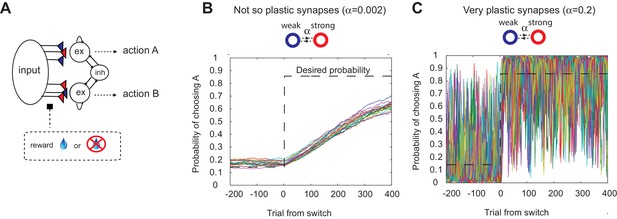
The decision making network and the speed accuracy tradeoff in synaptic learning.

(A) The decision making network. Decisions are made based on the competition (winner take all process) between the excitatory action selective populations, via the inhibitory population. The winner is determined by the synaptic strength between the input population and the action selective populations. After each trial, the synaptic strength is modified according to the learning rule. (B, C). The speed accuracy tradeoff embedded in the rate of synaptic plasticity. The horizontal dotted lines are the ideal choice probability and the colored lines are different simulation results under the same condition. The vertical dotted lines show the change points, where the reward contingencies were reversed. The choice probability is reliable only if the rate of plasticity is set to be very small ( $α = 0.002$ ); however, then the system cannot adjust to a rapid unexpected change in the environment (B). On the other hand, highly plastic synapses ( $α = 0.2$ ) can react to a rapid change, but with a price to pay as a noisy estimate afterwards (C).

https://doi.org/10.7554/eLife.18073.003

Figure 2

Download asset Open asset

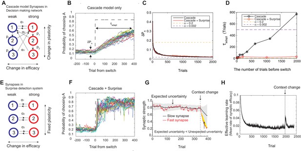
Our model solves the tradeoff the cascade model of metaplastic synapses guided by a surprise detection system.

(A) The cascade model of synapses for the decision making network. The synaptic strength is assumed to be binary (weak or strong); and there are multiple (three for each strength, in this example) meta-plastic states associated with these strengths. The transition probability of changing synaptic strength is denoted by $α_{i}$ , while the transition probability of changing plasticity itself is denoted by $p_{i}$ , where $α_{1} > α_{2} > \dots$ and $p_{1} > p_{2} > . . .$ . Deeper states are less plastic and less likely to enter. (B) The cascade model of synapses can reduce the fluctuation of estimation when the environment is stationary, thanks to the memory consolidation; however, the model fails to respond to a sudden change in the environment. (C) The changes in the fluctuation of choice probability in a stable environment. The cascade model synapses (black) can reduce the fluctuation gradually over time. This is also true when a surprise detection network (described below) is present. The dotted lines indicate the case with a single fixed plasticity that are used in Figure 1B,C. The probability fluctuation $δ P_{A}$ is defined as a mean standard deviation in the simulated choice probabilities. The synapses are assumed to be at the most plastic states at $t = 0$ . (D) The adaptation time required to switch to a new environment after a change point as a function of the size of the previous stable environment. The adaptation time increases proportionally to the duration of the previous stable environment for the cascade model (black). The surprise detection network can significantly reduce the adaptation time independent of the previous context length (red). The adaptation time $τ$ is defined as the number of trials required to cross the threshold probability ( $P_{A} = 0.7$ ) after the change point. (E) The simple synapses in the surprise detection network. Unlike the cascade model, the rate of plasticity is fixed, and each group of synapses takes one of the logarithmically segregated rates of plasticity $α_{i}$ ’s. (F) The decision making network with the surprise detecting system can adapt to an unexpected change. (G) How a surprise is detected. Synapses with different rates of plasticity encode reward rates on different timescales (only two are shown). The mean difference between the reward rates (expected uncertainty) is compared to the current difference (unexpected uncertainty). A surprise signal is sent when the unexpected uncertainty significantly exceeds the expected uncertainty. The vertical dotted line shows the change point, where the reward contingency is reversed. (H) Changes in the mean rates of plasticity (effective learning rate) in the cascade model with a surprise signal. Before the change point in the environment, the synapses become gradually less and less plastic; but after the change point, thanks to the surprise signal, the cascade model synapses become more plastic. In this figure, the network parameters are taken as $α_{i} = {(\frac{1}{5})}^{i}$ , $p_{i} = {(\frac{1}{5})}^{i}$ , $T = 0.1$ , $γ = 0$ , $m = 10$ , $h = 0.05$ , while the total baiting probability is set to $0.4$ and the baiting contingency is set to $9 : 1$ (VI schedule).

https://doi.org/10.7554/eLife.18073.004

Figure 3

Download asset Open asset

Our model captures key experimental findings and it shows a remarkable performance with little parameter tuning.

(A) The effective learning rate (red), defined by the average potentiation/depression rate weighted by the synaptic population on each state, changes depending on the volatility of the environment, consistent with key experimental findings in Behrens et al. (2007), Nassar et al. (2010). The learning rate gradually decreases over each stable condition, while it rapidly increases in response to a sudden change in environment. The grey vertical lines indicate the change points of contingencies. (B) The effective learning rate is self-tuned depending on the timescale of the environment. This contrasts the effective learning rate of our model (red line) to the harvesting efficiency if the model had a single-fixed rate of plasticity in a multi-armed bandit task with given block size (indicated by x-axis). The background colour shows the normalized harvesting efficiency of a single rate of plasticity model, which is defined by the amount of rewards that the model collected, divided by the maximum amount of rewards that the best model for each block size collected, so that the maximum is always equal to one. The median of the effective learning rate in each block is shown by the red trace, as the effective learning rate constantly changes over trials. The error bars indicate the 25th and 70th percentiles of the effective learning rates. (C) Our cascade model of metaplastic synapses can significantly outperform the model with fixed learning rates when the environment changes on multiple timescales. The harvest efficiency of our model of cascade synapses combined with surprise detection system (red) is significantly higher then the ones of the model with fixed learning rates, or the rates of plasticity (black). The task is a four-armed bandit task with blocks of 10 trials and 10,000 trials with the total reward rate $= 1$ . The total number of blocks is set to $1000 : 1$ . In a given block, one of the targets has the reward probability of $0.8$ , while the others have $0.2$ . The network parameters are taken as $α_{r}^{i} = {0.5}^{i}$ , $α_{n r}^{i} = {0.5}^{i + 1}$ , $p_{r}^{i} = {0.5}^{i}$ , $p_{n r}^{i} = {0.5}^{i + 1}$ , $T = 0.1$ , $γ = 1$ , $m = 12$ , $h = 0.05$ for (A), $α_{i} = p_{i} = {0.5}^{i}$ , $T = 0.1$ , $γ = 1$ , $m = 20$ , $h = 0.05$ for (B), $α_{i} = p_{i} = {0.5}^{i}$ , $T = 0.1$ , $γ = 1$ , $m = 4$ , $h = 0.0005$ for (C) , and $γ = 1$ and $T = 0.1$ for the single timescale model in (B).

https://doi.org/10.7554/eLife.18073.005

Figure 4

Download asset Open asset

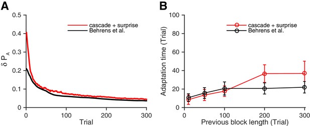
Our neural circuit model performs as well as a previously proposed Bayesian inference model (Behrens et al., 2007).

(A) Changes in the fluctuation of choice probability in a stable environment. As shown in previous figures, our cascade model synapses with a surprise detection system (red) reduces the fluctuation gradually over time. This is also the case for the Bayesian model (black). Remarkably, our model reduces the fluctuation as fast as the Bayesian model (Behrens et al., 2007). The probability fluctuation $δ P_{A}$ is defined as a mean standard deviation in the simulated choice probabilities. The synapses are assumed to be at the most plastic states at $t = 0$ , and uniform prior was assumed for the Bayesian model at $t = 0$ . (B) The adaptation time required to switch to a new environment after a change point. Again, our model (red) performs as well as the Bayes optimal model (black). Here the adaptation time $τ$ is defined as the number of trials required to cross the threshold probability ( $P_{A} = 0.6$ ) after the change point. The task is a 2-target VI schedule task with the total baiting rate of $= 0.4$ . The network parameters are taken as $α_{i} = {0.2}^{i}$ , $p_{i} = {0.2}^{i}$ , $T = 0.1$ , and $γ = 0$ , $m = 10$ , $h = 0.01$ . See Materials and methods, for details of the Bayesian model.

https://doi.org/10.7554/eLife.18073.006

Figure 5

Download asset Open asset

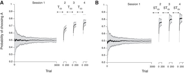
Our neural model with cascade synapses captures spontaneous recovery of preference (Mazur, 1996).

(A) Results for short inter-session-intervals (ISIs) (= 1 $T_{I S I}$ ). (B) Results for long ISIs (= 5 $T_{I S I}$ ). In both conditions, subjects first experience a long session (Session 1 with 3000 trials) with a balanced reward contingency, then following sessions (Sessions 2,3,4, each with 200 trials) with a reward contingency that is always biased toward target A (reward probability ratio: 9 to 1). Sessions are separated by ISIs, which we modeled as a period of forgetting according to the rates of plasticity in the cascade model (see Figure 7). As reported in (Mazur, 1996), the overall adaptation to the new contingency over sessions 2–4 was more gradual for short ISIs than long ISIs. Also, after each ISI the preference dropped back closer to the chance level due to forgetting of short timescales; however, with shorter ISIs subjects were slower to adapt during sessions. The task is a alternative choice task on concurrent VI schedule with the total baiting rate of 0.4. The mean and standard deviation of many simulation results are shown in Black line and gray area, respectively. The dotted horizontal lines indicate the target choice probability predicted by the matching law. The network parameters are taken as $α_{i} = {0.2}^{i}$ , $p_{i} = {0.2}^{i}$ , $T = 0.1$ , and $γ = 0$ , $m = 10$ , $h = 0.001$ .

https://doi.org/10.7554/eLife.18073.007

Figure 6

Download asset Open asset

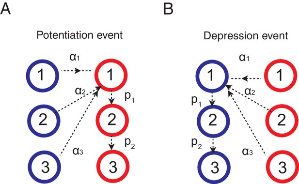
Learning rules for the cascade model synapses.

(A) When a chosen action is rewarded, the cascade model synapses between the input neurons and the neurons targetting the chosen action (hence those that with high firing rates) are potentiated with a probability determined by the current synaptic states. For those synapses at one of the depressed states (blue) would increase the strength and go to the most plastic, potentiated, state (red-1), while those at already one of the potentiated sates (red) would undergo metaplastic transitions (transition to deeper states) and become less plastic, unless they are already at the deepest state (in this example, state 3). (B) When an action is not rewarded, the cascade model synapses between the input population and the excitatory population targeting the chosen action are depressed with a probability determined by the current state. One can also assume an opposite learning for the synapses targeting the non-chosen action (In this case, we assume that all transition probabilities are scaled with $γ$ ).

https://doi.org/10.7554/eLife.18073.008

Figure 7

Download asset Open asset

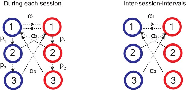
Forgetting during inter-session-intervals (ISIs).

In our simulations for the spontaneous recovery (Figure 5), we assumed that, during the ISI, random forgetting takes place in the cascade model synapses as shown on the right. As a result, synapses at more plastic states were more likely to be reset to the top states. This results in forgetting recent contingency but keeping a bias accumulated over a long timescale.

https://doi.org/10.7554/eLife.18073.009

Figure 8

Download asset Open asset

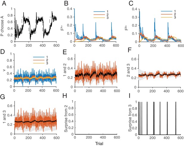
How the model works as a whole trial by trial.

Our model was simulated on a VI schedule with reward contingency being reversed every 100 trials (between $1 : 4$ and $4 : 1$ ). (A) The choice probability (solid line) generated from the decision making network. The dashed line indicates the target probability predicted by the matching law. The model’s choice probability nicely follows the ideal target probability. (B) The distribution of synaptic strength $F_{i}^{A^{+}}$ of the population targeting choice A. The different colors indicate different level of the depth $i = 1, 2, 3$ of synaptic states in the cascade model. The sum of these weights give the estimate of the value of choosing A. The shape rises in Blue are due to the surprise signals that were sent roughly every 100 trials due to the block change (see panel I). (C) The same for the other synaptic population $F_{i}^{B^{+}}$ targeting choice B. (D) The normalized synaptic strength $v_{i}$ in the surprise detection system that integrate reward history on multiple timescales. The numbers for different colors indicate synaptic population $i$ , with a fixed rate of plasticity $α_{i}$ . (E) The comparison of synaptic strengths $v_{i}$ between population 1 and 2. The black is the strength of slower synapses $v_{2}$ , while the red is the one of faster synapses $v_{1}$ . The gray area schematically indicates the expected uncertainty. (F) The comparison between $v_{2}$ and $v_{3}$ . (G) The comparison between $v_{2}$ and $v_{3}$ . (H) The presence of a surprise signal (indicated by 1 or 0, detected between $v_{1}$ and $v_{2}$ . There is no surprise since the unexpected uncertainty (red) was within the expected uncertainty (see E). (I) The presence of a surprise signal detected between $v_{1}$ and $v_{3}$ , or between $v_{2}$ and $v_{3}$ . Surprises were detected after each of sudden change in contingency (every 100 trials), mostly between $v_{2}$ and $v_{3}$ (see F,G). This surprise signal enhances the synaptic plasticity in cascade model synapses in the decision making circuit that compute the values of actions shown in B and C. This enables the rapid adaptation in choice probability seen in A The network parameters are taken as $α_{i} = {(\frac{1}{5})}^{i}$ , $p_{i} = {(\frac{1}{5})}^{i}$ , $T = 0.1$ , $γ = 0$ , $m = 10$ , $h = 0.01$ .

https://doi.org/10.7554/eLife.18073.010

Download links

A two-part list of links to download the article, or parts of the article, in various formats.

Downloads (link to download the article as PDF)

Article PDF

Open citations (links to open the citations from this article in various online reference manager services)

Mendeley

Cite this article (links to download the citations from this article in formats compatible with various reference manager tools)

Kiyohito Iigaya

(2016)

Adaptive learning and decision-making under uncertainty by metaplastic synapses guided by a surprise detection system

eLife 5:e18073.

https://doi.org/10.7554/eLife.18073

Sign up for email alerts

Privacy notice