Dynamics of embryonic stem cell differentiation inferred from single-cell transcriptomics show a series of transitions through discrete cell states
- Harvard University, United States
- Allen Institute for Brain Science, United States
Figures
Figure 1 with 1 supplement
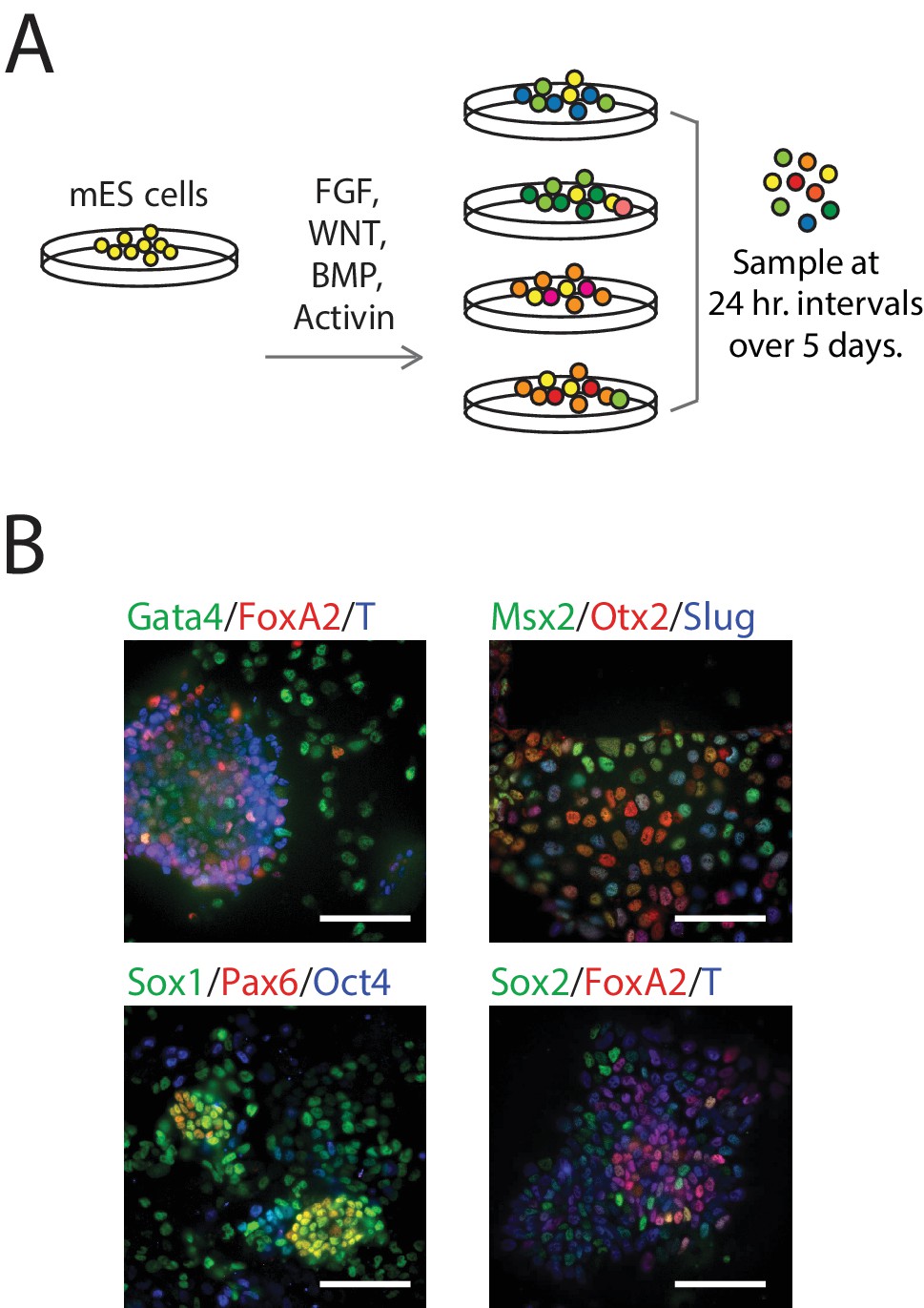
Single-Cell Gene Expression Profiling of mESCs during early germ layer differentiation.
(A) Mouse embryonic stem cells (mESCs) were exposed to various differentiation conditions to perturb FGF, WNT, and TGF-beta signaling for up to five days of differentiation. Single cells, collected every 24 hr during differentiation, were transcriptionally profiled using CEL-Seq. (See also Figure 1—figure supplement 1B and Figure 1—source data 1). (B) Images of immunostained mESCs undergoing differentiation show cell-to-cell variability in their expression of known germ layer marker genes. (Scale bar = 100 μm).
-
Figure 1—source data 1
Differentiation conditions and duration of single cells sorted into seven 96-well plates.
- https://doi.org/10.7554/eLife.20487.003
Figure 1—figure supplement 1
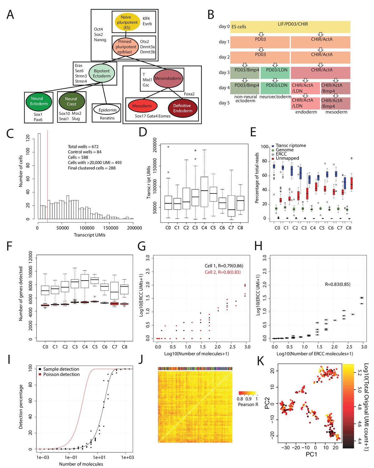
Quality validation of single-cell RNA-seq data.
(A) Diagram summarizing the literature on cell types (each represented by a colored circle labeled by its name) that arise during early mouse germ layer differentiation, their lineage relationships (represented by lines connecting cell types), and genes that characterize each cell type (listed in boxes that surround the cell types in which they are expressed). (B) Summary of cell culture conditions that were used to generate populations enriched with neural/non-neural ectoderm, definitive endoderm, or mesoderm-like cells over the course of up to five days. Undifferentiated ES cells were maintained in LIF/PD0/CHIR (i.e. Lif2i) conditions, and duration of differentiation was measured from the time at which these conditions were removed. (C) Histogram of the number of Unique Molecular Identifiers (UMIs) mapping to annotated genes per cell. Note that this histogram includes 84 control (empty or ERCC-only) wells. (D) Box and whisker plots of the number of UMIs mapping to annotated genes per cell, grouped by cell cluster (total cells = 288). (E) Percentage of reads mapping to the transcriptome, to the genome (i.e. regions outside the reference transcriptome annotation), and to ERCC spike-in control sequences, and percentage of reads unmapped per cell. Cells are grouped by cell cluster. (F) Box and whisker plots of the number of genes detected (UMI > 0) per cell, grouped by cluster, using the full data set (clear boxes) and after subsampling cells to 20,000 transcriptome-mapping UMIs (red boxes). (G) Representative plots for two cells, showing the number of UMIs detected for each ERCC species versus the putative number of molecules spiked in. UMI counts are based on subsampling to 20,000 transcriptome-mapping UMIs. Pearson’s R values in log space, using all ERCC species and using only ERCC species present at >1 molecule (in parentheses) are shown for each cell. (H) Same as E, but with mean and SEM values for all clustered cells, after subsampling to 20,000 transcriptome-mapping UMIs per cell. (I) Fraction of times a given ERCC species is detected (UMI > 0) in all clustered cells, after subsampling to 20,000 transcriptome-mapping UMIs per cell, versus the putative number of ERCC molecules spiked in. The red line indicates expected detection fractions based on Poisson statistics of dilution, whereas the black line indicates the best fit through the experimental data. The fit suggests that the detection rate is 1 out of 35 molecules. (J) Clustered heatmap of Pearson’s correlation coefficients among clustered cells based on ERCC UMI expression values. Clustering was done using average linkage with a distance metric of 1 – Pearson’s R. The color bar at the top identifies the cluster membership of each cell; cells of the same type do not cluster together based on ERCC expression, suggesting a lack of process-related artifacts in the final clusters. All box and whisker plots use boxes to represent the 25th and 75th percentile, and whiskers represent 1.5 times the intra-quartile range. (K) 288 cells (each dot is a cell) – colored by the total number of UMI reads – plotted against the first two principal components (x-axis, y-axis) of gene expression data calculated after subsampling 20,000 UMIs per cell. This shows that after subsampling 20,000 UMIs for each cell, cells do not show correlations based on read depth.
Figure 2 with 3 supplements
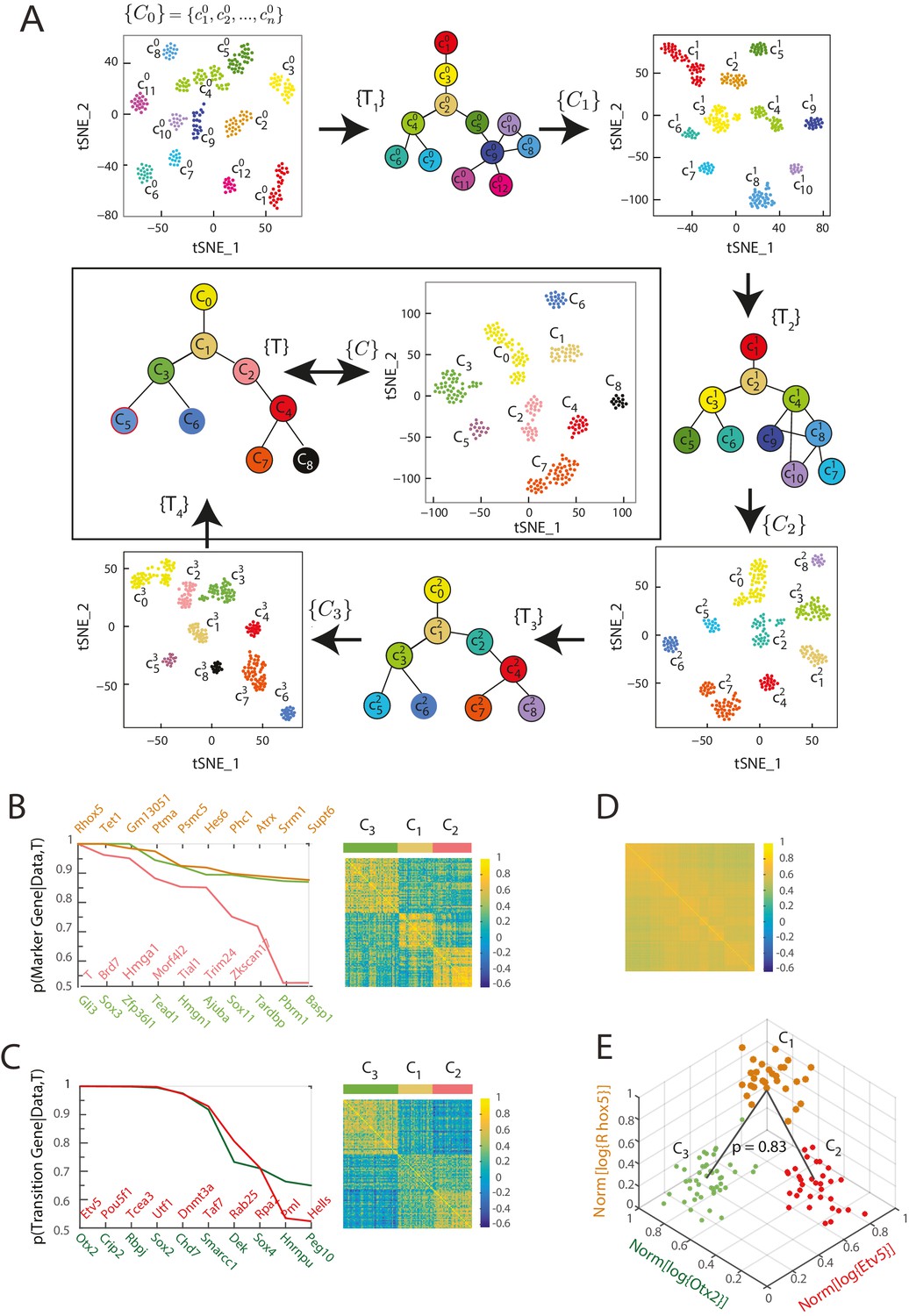
Iterative Bayesian algorithm converges upon a set of cell clusters and local transitions that together define a multi-potent lineage tree.
(A) Iterative determination of the most likely sets of transitions and re-clustering of cells in the resulting subspace of transition and marker genes, starting from a seed set of cluster identities . With each iteration, the cluster identities as well as the total number of clusters change, as shown by the Seurat t-SNE maps (each dot represents a cell, colored based on its cluster identity). The inferred sets of transitions between clusters at each iteration are represented as a lineage tree (each circle represents a cell cluster). After five iterations, the algorithm converged upon a set of 9 clusters (shown in box). (See also Figure 2—figure supplement 2). (B) Left: Top ten genes (x-axis) with highest probability of being marker genes for clusters C1 (yellow), C2 (light red) and C3 (light green) plotted against their probability of being marker genes. Right: Cell-cell correlation matrix computed using these 30 marker genes for the 108 cells belonging to clusters C1, C2 and C3 shows three clear blocks of high correlation along the diagonal. (C) Left: Top ten genes (x-axis) with highest probability of being transitioned genes for clusters C1, C2 and C3, plotted against their probability of being transitioned genes (y-axis). The transition genes belong to one of two classes, those that show high expression in cells belonging to C1 and C2 but low expression in C3 (red), and those expressed at high levels in cells in clusters C1 and C3 but low levels in C2 (green). The cell-cell correlation matrix computed using these 20 transition genes shows that the 29 cells belonging to cluster C1have intermediate levels of correlation with cells in both C2 and C3, whereas the 46 cells in C2 show low correlation levels with the 33 cells in C3. (D) The global cell-cell correlation matrix computed for all 288 cells using the 889 genes used for the final iteration of clustering shows a barely detectable structure. (E) The inferred clusters and their lineage relationships can be represented in a three-dimensional coordinate system where the x- and y- axes are the normalized log expression level of the two classes of transition genes (genes in Figure 2B, left) and the z-axis measures the normalized log expression level of the marker genes for cluster C1 (Figure 2A left in yellow). Each dot represents a single cell, and cells are colored based on their cluster identity.
-
Figure 2—source data 1
Plate and well id’s of cells belonging to each cluster.
- https://doi.org/10.7554/eLife.20487.006
-
Figure 2—source data 2
Triplet probabilities of final tree.
- https://doi.org/10.7554/eLife.20487.007
Figure 2—figure supplement 1
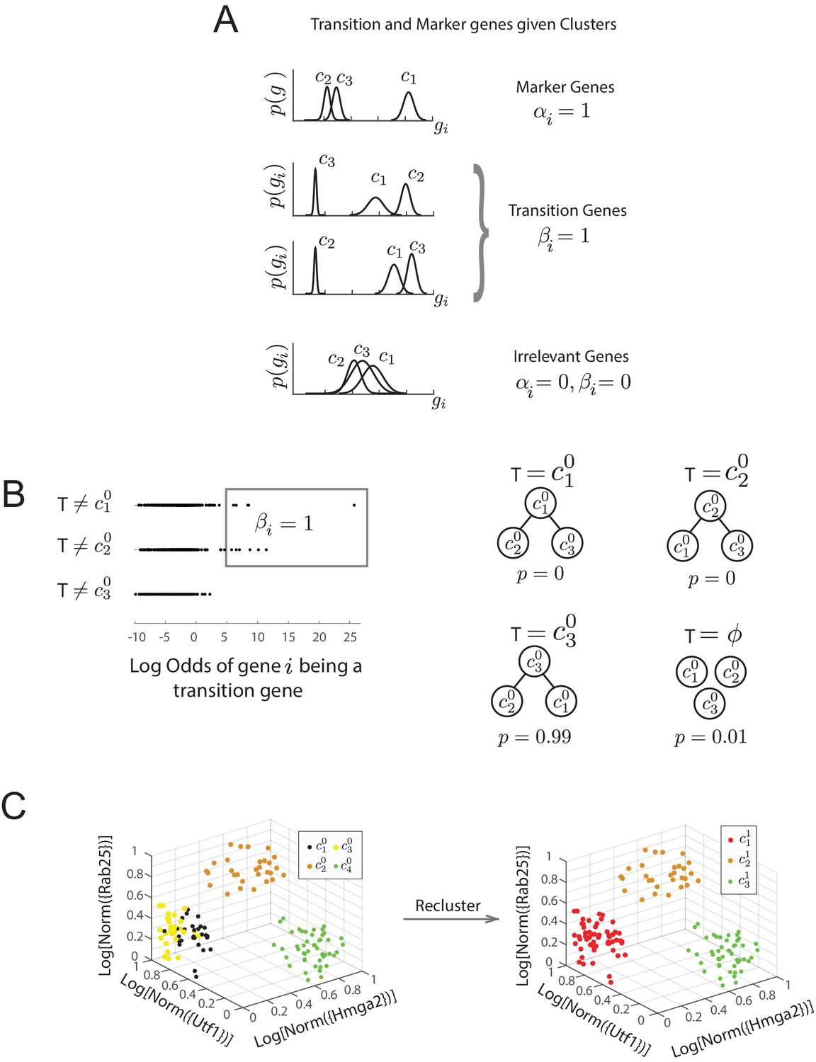
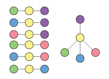
Diagram of Bayesian framework for inferring sequence of transitions for triplets.
(A) Gene expression patterns of marker genes, transition genes, and irrelevant genes in cell clusters c1, c2, and c3. Marker genes are highly expressed in only one cluster, whereas transition genes are highly expressed in two clusters and downregulated in the third. High probability transition genes alone are used for the determination of set of transitions; both high probability transition and marker genes are used for re-clustering. (B) For the three initial clusters , and , plot of the odds of each gene (represented by a dot) being a transition gene (x-axis) and the cluster with the minimum expression of the gene (y-axis). In our framework, each gene’s odds of being a transition gene is used to compute the probabilities of the sets of transitions between the three clusters (Furchtgott et al., 2016). A gene whose expression is lower in casts a probabilistic vote against being the intermediate state (i.e., against the relationships ), which is weighted by the odds that the gene is a transition gene, given the cluster identities. Two groups of genes (boxed) are the highest likelihood transition genes, casting a strong vote against or being the intermediate cell type. The computed probability of the topology given gene expression data indicates with. 99 probability that is the central node. (See also Materials and methods) (D) Left: single cells belonging to clusters (dots colored based on cluster identity) in the gene expression space defined by transition and marker genes (probability >0.8) associated with triplet , , . Axes represent the normalized log expression values of, respectively, transition genes expressed in and downregulated in and , and marker genes for ; the most likely gene of each class is represented in curly brackets. Right: after re-clustering cells in the subspace defined by high probability marker and transition genes, clusters and have merged.
Figure 2—figure supplement 2
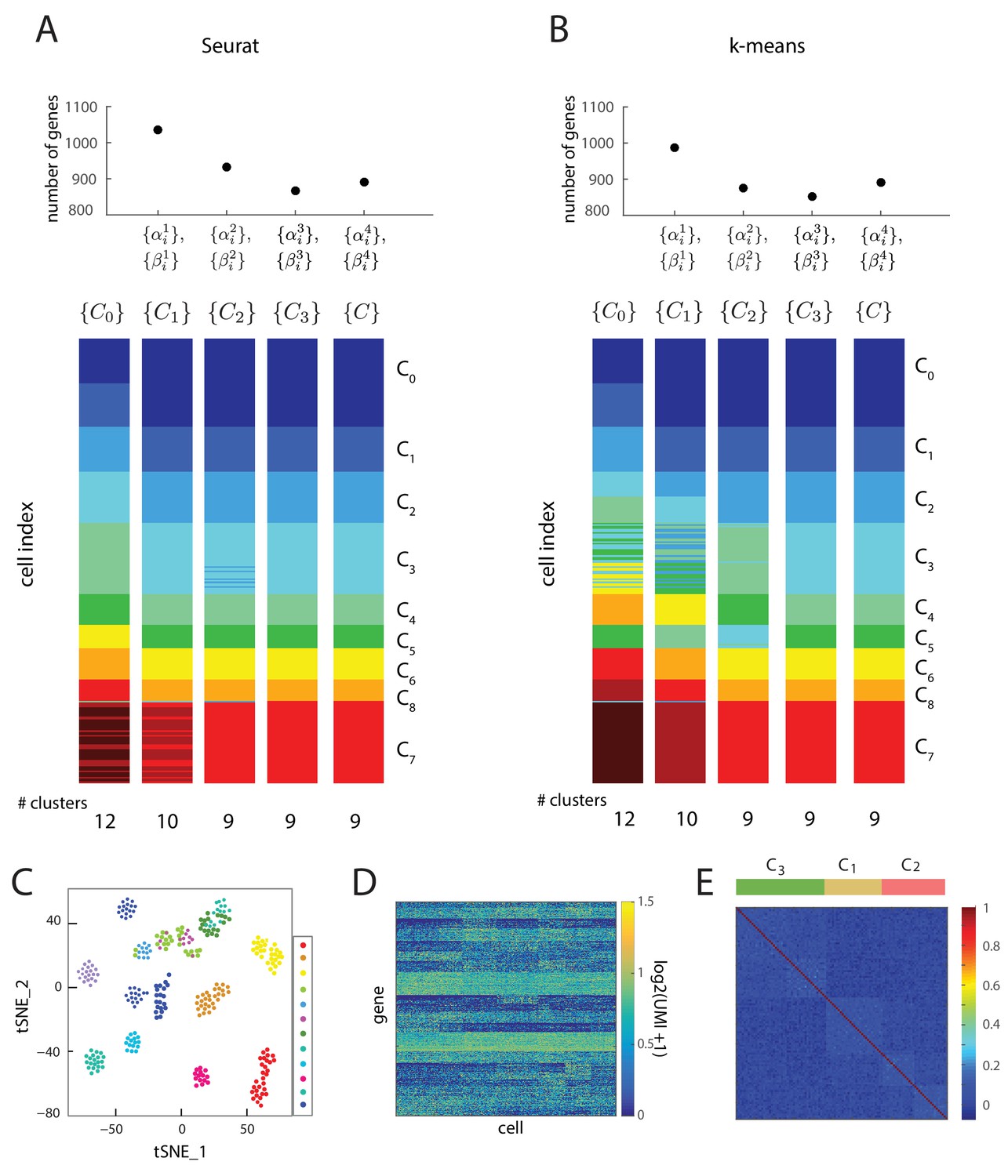
Iterative clustering and lineage determination is robust to clustering method.
(A, B) Iterative clustering and lineage determination algorithm using two different clustering methods for seed clusters and re-clustering: (A) Seurat, and (B) k-means clustering with the gap statistic. For each clustering method, the seed clusters were computed using the gene expression of all 2762 transcription factors. The top plot shows the number of marker and transition genes identified at each iteration and used for the subsequent re-clustering. The cluster identities for the single cells in different iterations are represented in different colors below. Despite starting with different seeds, both clustering methods converge to the same cluster identities after four iterations. (C) Two-dimensional projection of expression data from 288 single cells using Seurat. Each cell (single dot), colored by its cluster identity (there are 12 clusters in total), defined by k-means clustering, showing that t_SNE and k-means clustering lead to different seed cluster configurations. (D) Heat map showing the log-scale UMI of each of the 889 genes across all 288 cells. (E) The cell-cell correlation matrix computed using all genes with coefficient of variation greater than 10, which includes transition and marker genes, shows a barely-detectable signature of the underlying cell clusters (C1, C2 and C3) and the set of transitions between them.
Figure 2—figure supplement 3
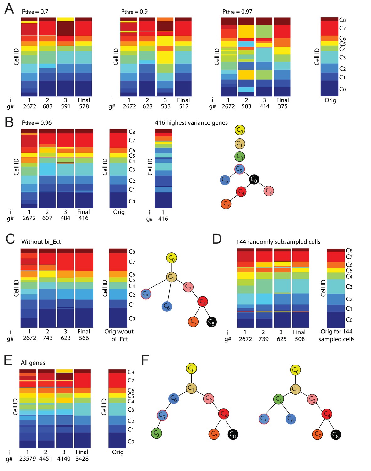
Iterative clustering and lineage determination is robust to changes in parameters.
(A) Iterative clustering and lineage determination is robust to changes in the threshold probability for determining whether a gene is a ‘high-probability’ transition or marker gene. Clustering configurations and lineage relationships that are inferred with a probability threshold of 0.7 (left) and 0.9 (middle-left) are identical to the original clustering configuration and lineage tree inferred with a threshold probability of 0.5 (rightmost column; lineage trees not shown). Each column corresponds to the cluster identities, represented by color, of all 288 cells (each row corresponds to one cell) for each iteration (i = 1, 2, 3 ...). The number of high-probability transition or marker genes (g#) used for clustering is shown below each iteration number. At a threshold of p=0.97 (middle-right), due to the number of genes used for re-clustering becoming ever smaller, the resulting clustering configuration shows several clusters merging or breaking into smaller clusters. (B) At a threshold of p=0.96 (left), the number of genes used for the last iteration of re-clustering (#g) is 416, which still results in a clustering configuration that is largely (>95%) identical to the original configuration. In contrast, the same number of highest-variance genes leads to a distinct clustering configuration (middle) as well as lineage tree given the original clustering configuration (right). (C, D) Iterative clustering and lineage determination is robust to changes in the set of cells. In the absence of C3 cells (C), the clustering identities (left) of the remaining cells and their lineage relationships (right) are unchanged. The same is true when a random subset of half of the 288 cells are omitted (D; lineage tree not shown). (E) Left: Iterative clustering and lineage determination using k-means clustering with all 23,579 genes for the seed cluster (i = 1) and resulting high-probability (p≥0.5) transition or marker genes for subsequent clustering iterations. Right: Original (described in Figure 2) final clustering configuration determined using only transcription factors. The clustering configuration is the same whether the gene pool is restricted to transcription factors or includes all genes. (F) The lineage trees inferred using all genes (left) and only transcription factors (right) have different ectoderm lineage topologies: the former assigns cluster C3 to be a descendent of C5 and C6 whereas the latter assigns C3 to be a common progenitor of C5 and C6. The mean differentiation duration is three days for C3 cells and four days for C5 and C6 cells (Figure 1—source data 1, Figure 2—source data 2), suggesting it is unlikely that C3 cells are descendants of C5 and C6 cells.
Figure 3 with 1 supplement
Cells transition from one discrete state to another during differentiation.
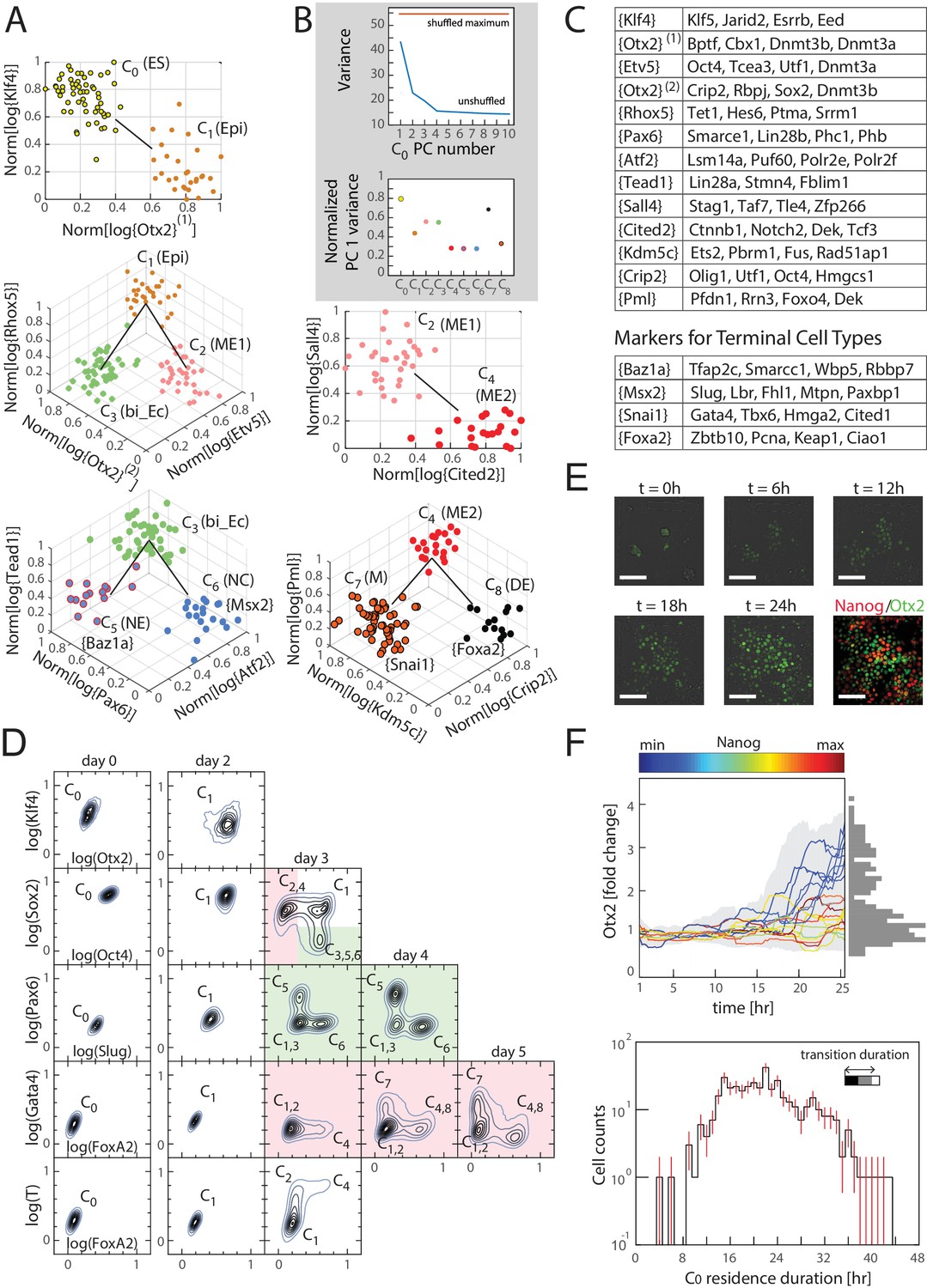
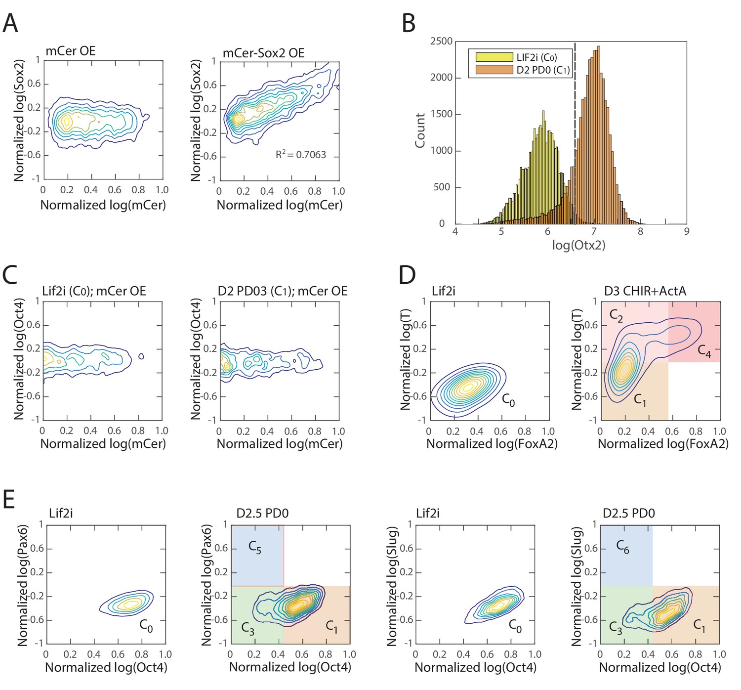
(A) Computationally inferred cell clusters and sequence of transitions are shown in the appropriate subspace of gene expression. Each dot represents a single cell, and cells are colored based on their cluster identity. For a linear transition sequence of cell states (such as from C0 to C1), the transitions are represented in a two dimensional plot with the axes defined by the normalized mean log of the unique reads of genes that are most differentially regulated in the two states, while for lineage bifurcations between alternative daughter cell states, the plots are shown in three dimensions, where the x and y axes are normalized mean log unique reads of the associated set of transition genes, and the z axes are the normalized mean log unique reads of the marker genes associated with the inferred progenitor state. Labeled in parenthesis next to each cluster are the abbreviated names of the putative corresponding cell types found in vivo (Epi: epiblast; bi_Ec: bi-potent ectoderm; ME: mesendoderm; NE: neural ectoderm; NC: neural crest; M: mesoderm; DE: definitive endoderm). (B) Top: Plot of the variances of the first ten principal components of the gene expression of cells in cluster C0. The red line is the maximum principal component variance over 1000 randomizations of the data, showing that no principal component is statistically significant. Bottom: variances of the first principal component of each cluster, normalized by the maximum principal component variance of the randomized gene expression data for the corresponding cluster. (C) A list of high probability genes that belong to the various marker and transition gene classes that define the axes of the plots in Figure 3A, each represented by one gene in curly brackets. The curly brackets contain the gene name with the highest probability for that class, and other high probability genes (as in Figure 2A and B) are listed in the table. While some of the genes are used only once, others such as Otx2 and Oct4 are repeatedly reused in different subspaces to describe the transition. (D) Flow cytometry analysis of cell populations sampled every 24 hr during differentiation and immunostained for nine genes (two shown at a time for each density contour plot): Klf4, Otx2, Oct4, Sox2, Slug, Pax6, FoxA2, Gata4 (each taken from a different gene class shown in Figure 3C), and T recapitulate the predicted structure and temporal ordering of transitions through discrete cell states. Axes represent the log of gene expression, normalized by the range between the minimum and maximum across each gene. Plots in pink and green represent C2 and C3 lineages following the split from C1, respectively. (E) Live cell microscopy of Otx2 reporter (mCitrine) cell line to infer the dynamics of cell state transition from C0 to C1. Sample images (shown) at t = 0, 6, 12, 18, and 24 hr of differentiation. Cells were terminated at approximately 25 hr into differentiation and immunostained for Nanog (ES marker gene, Figure 2—figure supplement 2A), which shows an anti-correlation between Otx2 and Nanog expression levels. (Scale bar = 100 μm) (F) Top: Time series (x-axis) traces of single-cell Otx2 (y-axis) expression dynamics taken every 15 min show that the duration of transition from Otx2-low (C0) to Otx2-high (C1) is approximately 4 hr, which is well within the time frame of one cell cycle (~10 hr). The end-point (t = 25 hr) Otx2 levels show a clear separation between high and low (histogram of ~200 cells shown to the right in gray), indicating that some cells have made the transition from C0 to C1 while others not. Each trace is colored by its relative end-point Nanog immunofluorescence intensity level. Otx2 levels are normalized by the mean level at t = 0. Bottom: Histogram (y-axis = log (cell count)) of residence durations of ~400 cells in the Otx2-low C0 state, showing that transition times vary across multiple cell cycle lengths (time lapse length = 48 hr). Inset bar shows mean as well as upper (white) and lower quartiles of the transition durations of cells.
-
Figure 3—source data 1
Probabilities of membership in marker and transition gene classes in final tree.
Listed are, for direct triplets along the lineage tree, the genes with the highest probabilities of belonging to transition gene and marker gene classes, and their associated probabilities. Genes belonging to the classes shown in curly brackets in Figure 3C (probability greater than 0.5%) are shown.
- https://doi.org/10.7554/eLife.20487.012
Figure 3—figure supplement 1
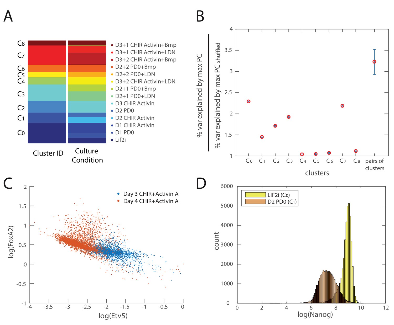
Validation of inferred cell types and lineage relationships.
(A) Comparison of clustering configuration (left column) and culture conditions (right column) shows that there is mixing of cells from different culture conditions to the same cluster as well as cells from the same culture conditions being assigned to different clusters. (B) Mean and coefficient of variation (c.v.) of percent variance explained by the largest eigenvalues of each cell cluster normalized by the percent variance explained by that of randomly shuffled gene expression data (y-axis) for each cell cluster (x-axis). The last point along the x-axis shows the mean and c.v. of percent variance explained by the largest eigenvalues of each cell cluster normalized by the percent variance explained by that of randomly shuffled data, for all merged pairs of cell clusters, which is significantly higher than that derived from single clusters (maximum p value . (C) A scatter plot of Etv5 (x-axis) and FoxA2 (y-axis) expression from immunofluorescence data (each dot is a mesendodermal cell, as identified by T expression; data not shown) shows that from day 3 to day 4 of mesendodermal differentiation (Materials and methods), Etv5 expression decreases and some cells go on to upregulate FoxA2. (D) Histogram of Nanog expression (as measured by immunostaining and flow cytometry) before differentiation (yellow; Lif2i C0 state) and after two days of differentiation (orange; D2 PD03 C1 state) shows that Nanog expression is downregulated throughout most of the population during the first two days, similar to the observed changes of Klf4 during this time (Figure 3D). We thus use Nanog immunostaining, which produces a better signal compared to Klf4 antibodies, to identify cells that are still remaining in the naïve pluripotent C0 state.
Figure 4 with 3 supplements

Quantitative modeling of the network underlying germ layer differentiation.
(A) The inferred gene regulatory network from 10,000 sampled solutions that stabilize each of the nine cell states. Each circle represents a gene module. Mean positive and negative interactions between the modules are shown in red and green, respectively, and their thickness and transparency are proportional to the absolute magnitude of the mean and the coefficient of variation (c.v.), respectively. The colored circles represent the gene modules expressed uniquely in only one of the cell states (color code matched with Figure 3A for each state). (B, C) Subsets of the network consisting of gene modules that are expressed in (and stabilize) the naïve ES C0 state (B) and epiblast-like C1 (C) state. As cells transition from C0 to C1, expression of [Klf4], [Apex1], [Ets2], [Atf2] modules is downregulated (shown in gray) while [Hes6] and [Otx2] modules are upregulated, leading to changes in the effective interactions between gene modules that are common to both C0 and C1 states, such as [Sox2] and [Oct4]. (D) [Sox2] overexpression (x-axis) plotted against the probability of [Oct4] downregulation (y-axis) computed over 10,000 models (Materials and methods). In the C1 state (solid line), [Oct4] is downregulated in an increasing fraction of models following [Sox2] overexpression, while in C0, [Oct4] is stable in ~96% of the models (dotted line). In order to obtain the error bars for this and subsequent predictions, we randomly sampled three subsets of 3333 from the 10,000 models. For each set we computed the mean and standard error of the proportion of models that show downregulation of Oct4 in response to Sox2 overexpression. (E, F) Subsets of the model consisting of gene modules that are expressed in the epiblast-like C1 (E) and mesendoderm-like C2 (F) states, and their interactions with [Snai1], which is not normally expressed in C1 or C2. As cells transition from the C1 to C2 state, [Hes6], [Sox2], [Otx2], [Churc1] are downregulated (shown in gray), while [Hmga1], [T], [Atf2], [Hes1], [Ets2], [Apex1], [Brd7], [Hmgn2] and [Smarce1] are upregulated, leading to changes in the effective interactions between [Snai1] and modules that are common to both C1 and C2, such as [Oct4]. (G) The probability of [Oct4] being downregulated (y-axis) as a function of [Snai1] overexpression (x-axis). In the C1 state (solid line), the over expression of [Snai1] has no effect on [Oct4] levels in ~94.5% of the 10,000 models whereas in the C2 state (dotted line), the overexpression of [Snai1] leads to [Oct4] downregulation in up to 19% of the models. (H) The C3 state shows a downregulation of [Oct4] and [BMP], and upregulation of [Tead1], [Apex1], [Pax6], [Smarce1], [Ets2], [Atf2], [Hes1], [Fhl1], [Hmgn2] modules relative to C1. (I) Cells in different states are predicted to respond differently to morphogens. Plot showing the percentage of models (y-axis) where states C1 and C3 (x-axis) transition to C6 (characterized by unique marker gene module [Msx2]), in response to [LIF]+[BMP]. C1 cells remain stable in response to [LIF]+[BMP] signaling in >98% of the models whereas C3 cells are destabilized and move to the C6 state in ~11% of the models.
-
Figure 4—source data 1
Gene modules used for modeling the network.
* The [BMP] and [Aes] modules have the same binary pattern. ** The [FGF] and [WNT] modules have the same binary pattern.
- https://doi.org/10.7554/eLife.20487.015
-
Figure 4—source data 2
Binary expression profiles of the gene modules used for modeling the network in the 9 cell clusters.
- https://doi.org/10.7554/eLife.20487.016
Figure 4—figure supplement 1
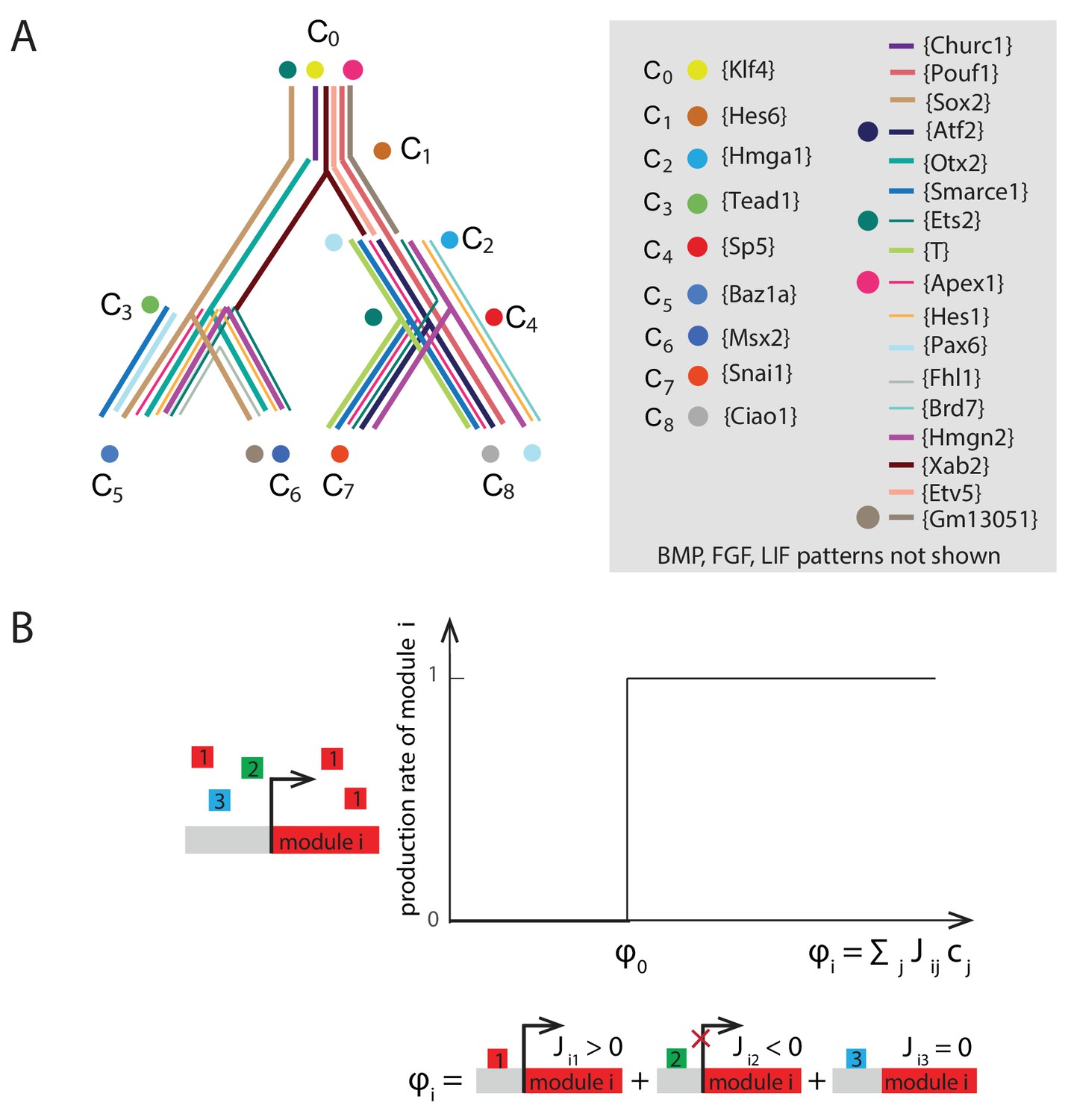
Summary of gene modules and illustration of production rate determination for each gene module.
(A) River diagram of the gene expression patterns of the 29 modules in the 9 cell clusters. Straight lines indicate asymmetric regulation favoring the colored branch; dots indicate symmetric downregulation in the subsequent two branches. (B) Plot of the production rate of module , , as a function of the drive from the other modules . The production rate is equal to 1 if the drive is greater than a critical drive and 0 otherwise.
Figure 4—figure supplement 2
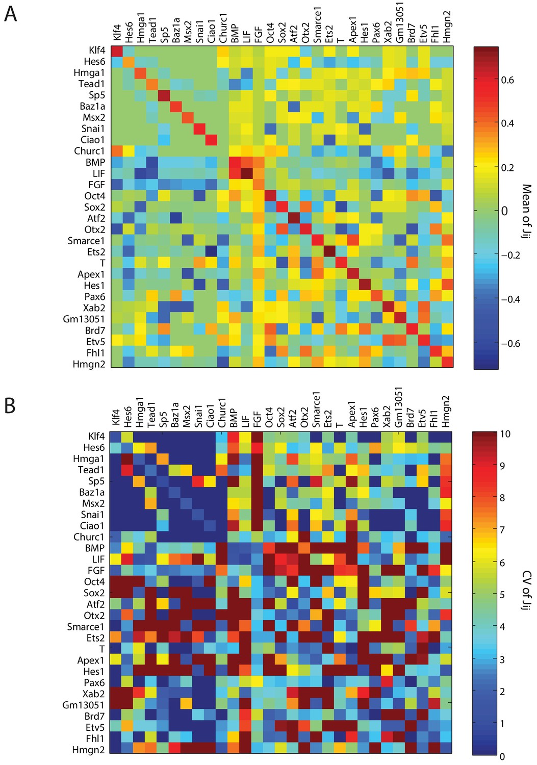
Summary of parameters for model gene regulatory network.
(A, B) Heat maps showing the absolute mean (A) and coefficient of variation (c.v.) (B), of the 841 parameters of the inferred gene regulatory network from 10,000 sampled solutions that stabilize each of the nine cell states. The (i,j)- th element of the each of the matrices shows the mean (A) and c.v (B) of the interaction strength , in which gene module j exerts a drive on gene module i.
Figure 4—figure supplement 3
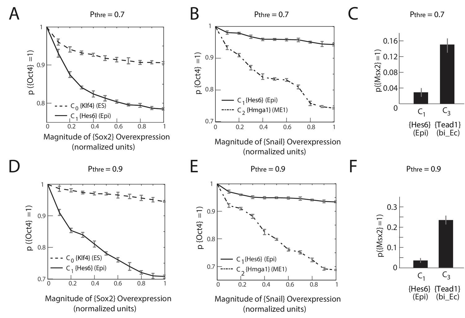
The predictions of the gene regulatory network are robust to changes in the probability threshold for considering a gene to be a transition or a marker gene.
For a probability threshold of 0.7 (A, B, C) and 0.9 (D, E, F), we obtain 27 and 24 different gene modules, respectively. (A, D) [Sox2] overexpression (x-axis) plotted against the proportion of models where [Oct4] remains high (i.e., binarized value equals 1) (y-axis) computed over 10,000 models. In the C1 state (solid line), [Oct4] is downregulated in an increasing fraction of models following [Sox2] overexpression relative to when [Sox2] is overexpressed in the C0 state (dotted line). (B, E) [Snai1] overexpression (x-axis) plotted against the proportion of models where [Oct4] is high (y-axis) computed over 10,000 models. [Oct4] is downregulated in an increasing fraction of models following [Snai1] overexpression in the C2 state (dotted line) relative to when [Snai1] is overexpressed in the C1 state (solid line). (C, F) C1 cells remain more stable in response to [LIF]+[BMP] signaling relative to C3 cells, which move to the C6 state in a significantly higher fraction of the models.
Figure 5 with 1 supplement
Experimental validation shows that interpretation of Sox2, Snai1, and LIF+BMP is cell state dependent.
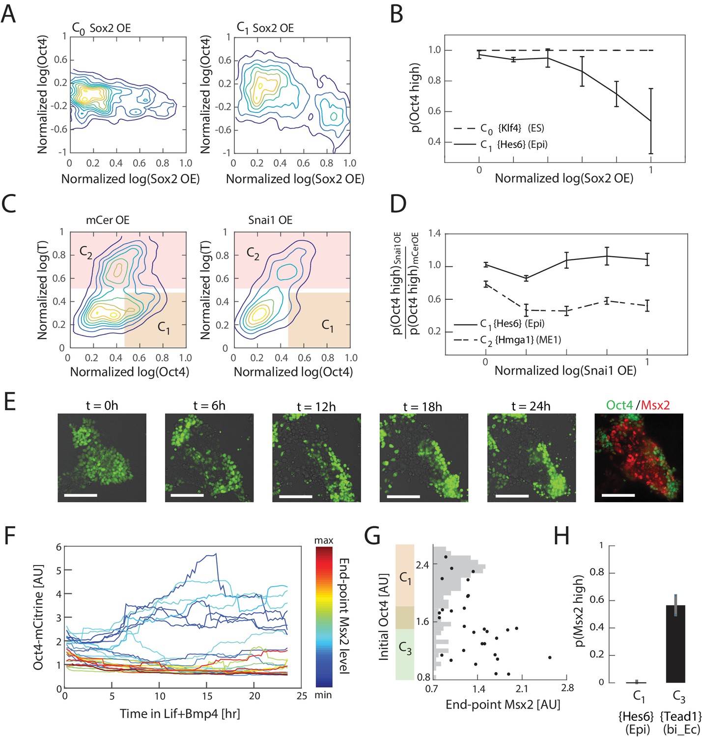
(A) Comparison of the effects of Sox2 overexpression (x-axis) on Oct4 levels (y-axis) in the naïve ES state C0 (left) and epiblast-like C1 state shows negative correlation between Sox2 overexpression and Oct4 levels in the C1 state, but not in C0. Plots showing mCerulean (marker) -only overexpression in C0 or C1 are indistinguishable from Sox2 overexpression in C0 (Figure 5—figure supplement 1C). (B) Fraction of Oct4-high cells (y-axis; defined as greater than 2σ below the mean log of Oct4 of non-transfected control cells) plotted against binned Sox2 overexpression level confirms model prediction (Figure 4D) that Sox2 overexpression leads to downregulation of Oct4 in C1 but not C0. (C) Comparison of the effects of Snai1 and mCerulean-only (left) overexpression on Oct4 levels (x-axis) in the epiblast-like C1 and mesendoderm-like C2 states (y-axis; T-low and –high, respectively) shows downregulation of Oct4 in response to Snai1 overexpression in the C1 state but not in C2. (D) Fraction of Oct4-high cells in Snai1 overexpressing cells, normalized by this fraction in mCerulean overexpressing control cells (y-axis), plotted against binned Snai1 overexpression level (x-axis) confirms the prediction (Figure 4G) that Snai1 overexpression leads to greater downregulation of Oct4 in C2 compared to C1. (E) Live cell images of Oct4-mCitrine cells at t = 0, 6, 12, 18, 24 hr of LIF+BMP exposure. At t = 0, cells are either in state C1 (Oct4-high) or C3 (Oct4-low) (Figure 5—figure supplement 1E). (Scale bar = 100 μm) Cells were fixed at t = 24 hr and immunostained for Msx2. (F) Time series (x-axis) traces of single-cell Oct4 expression (y-axis) taken every 15 min from live cells. Each trace is colored by its relative end-point Msx2 immunofluorescence intensity level. (G) The initial Oct4 reporter (mCitrine) intensity (y-axis) and final Msx2 immunofluorescence (x-axis) are negatively correlated. Each dot represents a single cell. Histogram of Oct4 reporter intensity at t = 0 levels shown in gray. Based on this histogram, we defined a range of threshold values for determining Oct4-high and –low (shown in overlapping region of orange and green along y-axis). (H) Plot showing fraction of Msx2-high (y-axis; as defined by greater than 2σ above background) confirms prediction (Figure 4I) that Msx2 is upregulated with a greater probability in the C3 state compared to C1 (x-axis) in response to LIF+BMP exposure.
Figure 5—figure supplement 1
Controls for perturbation experiments.
(A) mCerulean fluorescence level correlates with increasing total Sox2 levels, validating the use of mCerulean fluorescence as a measure for Sox2 overexpression. (Left) As a control, we show that Sox2 levels do not increase when only mCerulean is overexpressed. (B) Histogram of Otx2 expression (as measured by immunostaining and flow cytometry) following 24 hr of Sox2 overexpression in either naïve ES C0 cells (Lif2i; yellow) or epiblast-like C1 cells (D2 PD0; orange). In determining the effects of Sox2 overexpression in the epiblast-like C1 state (Figure 5A), we excluded cells that showed Otx2 expression less than two standard deviations above the mean of Otx2 levels in Lif2i (threshold shown in dotted line). (C) Overexpression of only mCerulean does not show any effect on Oct4 levels in both C0 (left; Lif2i) and C1 (right; D2 PD0) cell states. (D) At day 3 of differentiation using CHIR99021 and Activin A (Materials and methods), populations consist of cells in C1 (FoxA2-low, T-low) C2 (FoxA2-low, T-high) and C4 (FoxA2-high, T-high) states. The fraction of cells in C4 is 17%. FoxA2 and T levels in undifferentiated C0 state cells (Lif2i) are shown as a reference (left). (E) At day 2.5 of differentiation using PD0325901 (Materials and methods), populations consist of cells in C1 (Oct4-high) and C3 (Oct4-low) states. At this point cells have not yet upregulated Pax6 (left two panels) or Slug (right two panels), showing that cells have not yet transitioned to either state C5 or C6.
Author response image 1
Download links
A two-part list of links to download the article, or parts of the article, in various formats.
Downloads (link to download the article as PDF)
Open citations (links to open the citations from this article in various online reference manager services)
Cite this article (links to download the citations from this article in formats compatible with various reference manager tools)
Dynamics of embryonic stem cell differentiation inferred from single-cell transcriptomics show a series of transitions through discrete cell states
eLife 6:e20487.
https://doi.org/10.7554/eLife.20487


