On cross-frequency phase-phase coupling between theta and gamma oscillations in the hippocampus
Figures
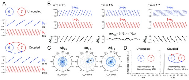
Measuring cross-frequency phase-phase coupling.
(A) Traces show 500 ms of the instantaneous phase time series of two Kuramoto oscillators (see Materials and methods). When uncoupled (top panels), the mean natural frequencies of the ‘theta’ and ‘gamma’ oscillator are 8 Hz (blue) and 43 Hz (red), respectively. When coupled (bottom panels), the oscillators have mean frequencies of 8.5 Hz and 42.5 Hz. (B) Top blue traces show the instantaneous phase of the coupled theta oscillator for the same period as in A but accelerated m times, where m = 3 (left), 5 (middle) and 7 (right). Middle red traces reproduce the instantaneous phase of the coupled gamma oscillator (i.e., n = 1). Bottom black traces show the instantaneous phase difference between gamma and accelerated theta phases (). Notice roughly constant only when theta is accelerated m = 5 times, which indicates 1:5 phase-locking. See Figure 1—figure supplement 1 for the uncoupled case. (C) distributions for the coupled case (epoch length = 100 s). Notice uniform distributions for n:m = 1:3 and 1:7, and a highly concentrated distribution for n:m = 1:5. The black arrow represents the mean resultant vector for each case (see Materials and methods). The length of this vector (Rn:m) measures the level of n:m phase-locking. See Figure 1—figure supplement 1 for the uncoupled case. (D) Phase-locking levels for a range of n:m ratios for the uncoupled (left) and coupled (right) oscillators (epoch length = 100 s).
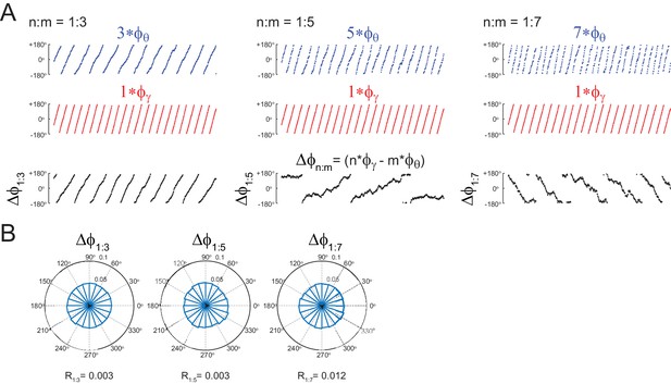
Uncoupled oscillators display uniform distribution.
(A,B) Panels show the same as in Figure 1B,C, but for the uncoupled oscillators. Notice roughly uniform distributions.
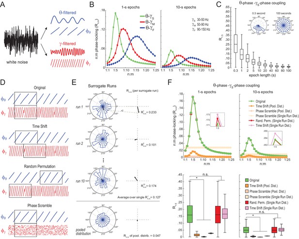
Detection of spurious n:m phase-locking in white-noise signals due to inappropriate surrogate-based statistical testing.
(A) Example white-noise signal (black) along with its theta- (blue) and gamma- (red) filtered components. The corresponding instantaneous phases are also shown. (B) n:m phase-locking levels for 1- (left) and 10 s (right) epochs, computed for noise filtered at theta (θ; 4–12 Hz) and at three gamma bands: slow gamma (γS; 30–50 Hz), middle gamma (γM; 50–90 Hz) and fast gamma (γF; 90–150 Hz). Notice Rn:m peaks in each case. (C) Boxplot distributions of θ−γS R1:5 values for different epoch lengths (n = 2100 simulations per epoch length). The inset shows representative distributions for 0.3- and 100 s epochs. (D) Overview of surrogate techniques. See text for details. (E) Top panels show representative distributions for single surrogate runs (Time Shift; 10 runs of 1 s epochs), along with the corresponding Rn:m values. The bottom panel shows the pooled distribution; the Rn:m of the pooled distribution is lower than the Rn:m of single runs (compare with values for 1- and 10 s epochs in panel C). (F) Top, n:m phase-locking levels computed for 1- (left) or 10 s (right) epochs using either the Original or five surrogate methods (insets are a zoomed view of Rn:m peaks). Bottom, R1:5 values for white noise filtered at θ and γS. Original Rn:m values are not different from Rn:m values obtained from single surrogate runs of Random Permutation and Time Shift procedures. Less conservative surrogate techniques provide lower Rn:m values and lead to the spurious detection of θ−γS phase-phase coupling in white noise. *p<0.01, n = 2100 per distribution, one-way ANOVA with Bonferroni post-hoc test.
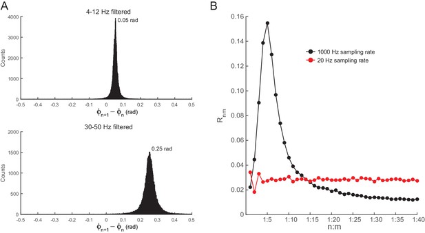
Filtering induces quasi-linear phase shifts in white-noise signals.
(A) Distribution of the phase difference between two consecutive samples for white noise band-pass filtered at theta (4–12 Hz, top) and slow gamma (30–50 Hz, bottom). Epoch length = 100 s; sampling rate = 1000 Hz (dt = 0.001 s). Notice that the top histogram peaks at ~0.05, which corresponds to 2*3.14*8*0.001 (i.e., 2*π*fc*dt, where fc is the center frequency), and the bottom histogram peaks at ~0.25 =2*3.14*40*0.001. (B) Rn:m curves computed for theta- and slow gamma-filtered white-noise signals. The black curve was obtained using continuous 1 s long time series sampled at 1000 Hz. The red curve was obtained by also analyzing 1000 data points, but which were subsampled at 20 Hz (subsampling was performed after filtering). Notice Rn:m peak at n:m = 1:5 only for the former case. See also Figure 5—figure supplement 7 for similar results in hippocampal LFPs.
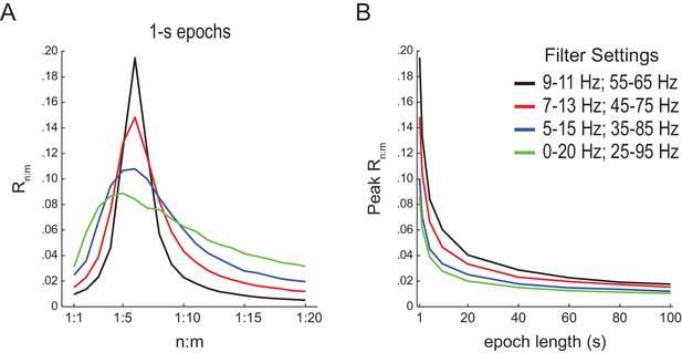
Filter bandwidth influences n:m phase-locking levels in white-noise signals.
(A) Mean Rn:m curves computed for 1 s long white-noise signals filtered into different bands (same color labels as in B; n = 2100). Notice that the narrower the filter bandwidth, the higher the Rn:m peak. (B) Mean Rn:m peak values for different filter bandwidths and epoch lengths (n = 2100 simulations per filter setting and epoch length).

Uniform p-value distributions upon multiple testing of Original Rn:m values against Single Run Rn:m surrogates.
The histograms show the distribution of p-values (bin width = 0.02) for 10000 t-tests of Original Rn:m vs Single Run surrogate values (n = 30 samples per group; epoch length = 1 s). The red dashed line marks p=0.05. The p-value distributions do not statistically differ from the uniform distribution (Kolmogorov-Smirnov test).
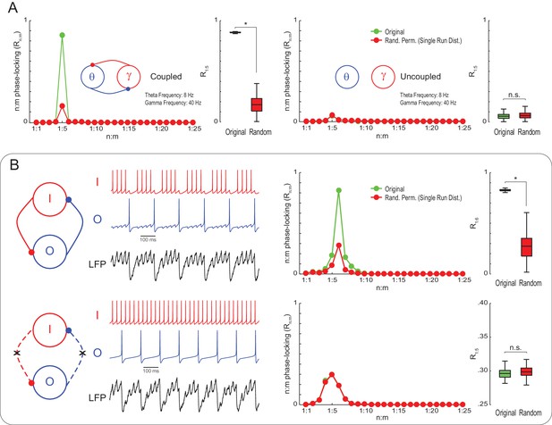
True n:m phase-locking leads to significant Rn:m values.
(A) The left panels show mean Rn:m curves and distributions of R1:5 values for original and surrogate (Random Permutation/Single Run) data obtained from the simulation of two coupled Kuramoto oscillators (n = 300; epoch length = 30 s; *p<0.001, t-test). The right panels show the same, but for uncoupled oscillators. In these simulations, each oscillator has instantaneous peak frequency determined by a Gaussian distribution; the mean natural frequencies of the theta and gamma oscillators were set to 8 Hz and 40 Hz, respectively (coupling does not alter the mean frequencies since they already exhibit a 1:5 ratio; compare with Figure 1). (B) Top panels show results from a simulation of a model network composed of two mutually connected interneurons, O and I cells, which emit spikes at theta and gamma frequency, respectively (Tort et al., 2007; Kopell et al., 2010). Original n:m phase-locking levels are significantly higher than chance (n = 300; epoch length = 30 s; *p<0.001, t-test). The bottom panels show the same, but for unconnected interneurons. In this case, n:m phase-locking levels are not greater than chance.
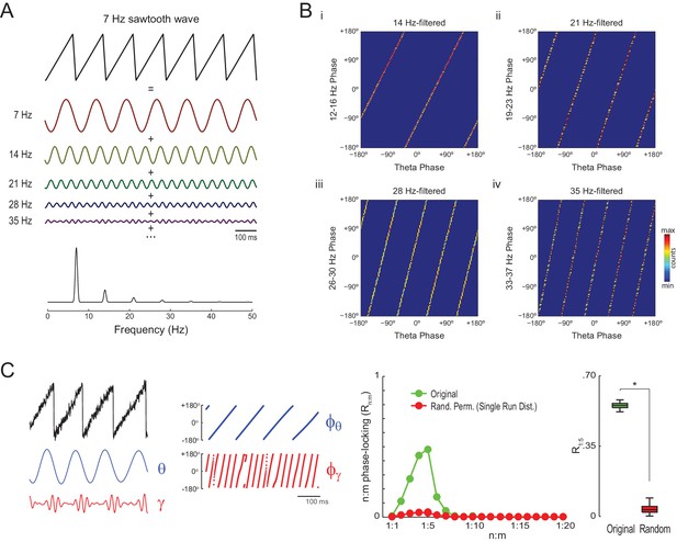
Waveform asymmetry may lead to artifactual n:m phase-locking.
(A) The top traces show a theta sawtooth wave along with its decomposition into a sum of sinusoids at the fundamental (7 Hz) and harmonic (14 Hz, 21 Hz, 28 Hz, 35 Hz, etc) frequencies. The bottom panel shows the power spectrum of the sawtooth wave. Notice power peaks at the fundamental and harmonic frequencies. (B) Phase-phase plots (2D histograms of phase counts) for the sawooth wave in A filtered at theta (7 Hz; x-axis phases) and harmonic frequencies (14, 21, 28 and 35 Hz; y-axis phases). (C) The left traces show 500 ms of a sawtooth wave along with its theta- and gamma-filtered components and corresponding phase time series. The sawtooth wave was set to have a variable peak frequency, with mean = 8 Hz; no gamma oscillation was added to the signal. Notice that the sharp deflections of the sawtooth wave give rise to artifactual gamma oscillations in the filtered signal (Kramer et al., 2008), which have a consistent phase relationship to the theta cycle. The right panels show that artifactual n:m phase-coupling levels induced by the sharp deflections are significantly higher than the chance distribution (n = 300; epoch length = 30 s; *p<0.001, t-test).
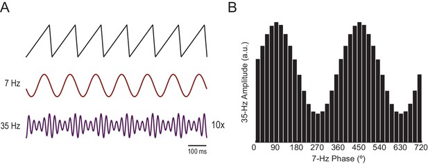
Waveform asymmetry may lead to spurious phase-amplitude coupling.
(A) A theta sawtooth wave along with its theta- (7 Hz) and gamma-filtered (35 Hz) components. Notice that no gamma oscillations exist in the original sawtooth wave, but they spuriously appear when filtering sharp deflections (Kramer et al., 2008). The amplitude of the spurious gamma waxes and wanes within theta cycles. (B) Mean gamma amplitude as a function of theta phase.
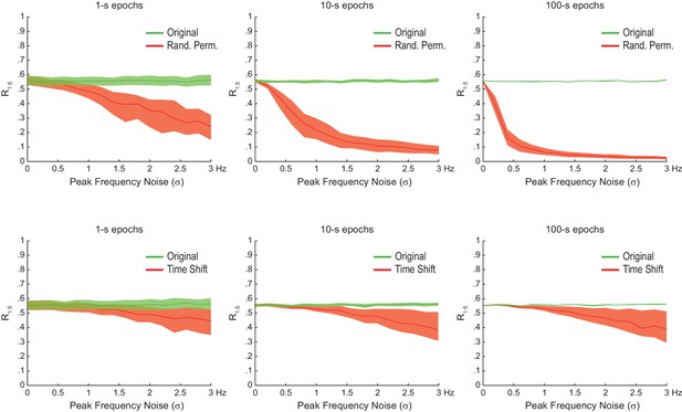
The statistical significance of artifactual n:m phase-locking levels induced by waveform asymmetry depends on epoch length and peak frequency variability.
Shown are the median R1:5 computed between theta and slow gamma for sawtooth waves simulated as in Figure 4C, but of different epoch lengths and peak frequency variability. Dashed area corresponds to the interquartile range (n = 300). Surrogate data were obtained either by Radom Permutation (top row) or Time Shift (bottom row) procedures. Notice that the longer the epoch or the peak frequency variability, the larger the difference between original and surrogate data, and that this difference is greater for randomly permutated than time-shifted surrogates.
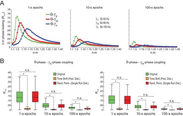
Spurious detection of theta-gamma phase-phase coupling in the hippocampus.
(A) n:m phase-locking levels for actual hippocampal LFPs. Compare with Figure 2B. (B) Original and surrogate distributions of Rn:m values for slow (R1:5; left) and middle gamma (R1:8; right) for different epoch lengths. The original data is significantly higher than the pooled surrogate distribution, but indistinguishable from the distribution of surrogate values computed using single runs. Similar results hold for fast gamma. *p<0.01, n = 7 animals, Friedman’s test with Nemenyi post-hoc test.
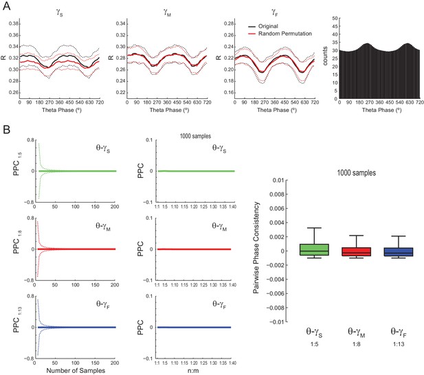
Lack of evidence for cross-frequency phase-phase coupling between theta and gamma oscillations using alternative phase-locking metrics.
(A) The left plots show the mean radial distance (R) computed for gamma phases in different theta phase bins, as described in Sauseng et al. (2009). The lines denote the mean ± SD over all channels across animals (n = 16 channels per rat x seven rats); 300 1 s long epochs were analyzed for each channel. Note that original and surrogate R values overlap. The variations of R values within a theta cycle are explained by the different number of theta phase bins (right bar plot), which leads to different number of analyzed samples; the higher the number of analyzed samples, the lower the R (see also Figure 2C). (B) The first column shows the mean pairwise phase consistency (PPC) between gamma and accelerated theta phases as a function of the number of samples (dashed lines denote SD over individual PPC estimates; n = 112 channels x 1000 PPC estimates per channel). Since PPC requires independent observations (Vinck et al., 2010), was randomly sampled to avoid the statistical dependence among neighboring data points imposed by the filter (Figure 2—figure supplement 1; see also Figure 5—figure supplement 7). The second column shows mean PPC as function of n:m ratio (individual PPC estimates were computed using 1000 samples); the boxplot distributions show PPC values at selected n:m ratios, as labeled. PPC values are very low for all analyzed frequency pairs and not statistically different from zero.
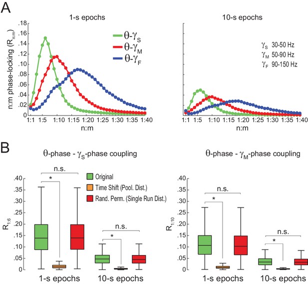
Spurious detection of theta-gamma phase-phase coupling when theta phase is estimated by interpolation.
(A) n:m phase-locking levels for actual hippocampal LFPs (same dataset as in Figure 5). Theta phase was estimated by the interpolation method described in Belluscio et al. (2012). (B) Original and surrogate distributions of Rn:m values. The original data are significantly higher than surrogate values obtained from pooled , but indistinguishable from single run surrogates. *p<0.01, n = 7 animals, Friedman’s test with Nemenyi post-hoc test.
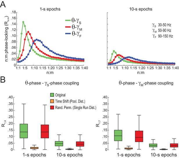
Spurious detection of theta-gamma phase-phase coupling (second dataset).
(A) n:m phase-locking levels for actual hippocampal LFPs. (B) Original and surrogate distributions of Rn:m values. Results obtained for three rats recorded in an independent laboratory (see Materials and methods).
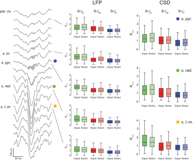
Lack of evidence for theta-gamma phase-phase coupling in all hippocampal layers.
(Left) Example estimation of the anatomical location of a 16-channel silicon probe by the characteristic depth profile of sharp-wave ripples (inter-electrode distance = 100 μm). (Middle) Original and surrogate (Random Permutation/Single Run) distributions of Rn:m values computed between theta phase and the phase of three gamma sub-bands (1 s long epochs). Different rows show results for different layers. (Right) Distribution of original and surrogate Rn:m values computed for current-source density (CSD) signals (1 s long epochs) in three hippocampal layers: s. pyramidale (top), s. radiatum (middle), and s. lacunosum-moleculare (bottom). Notice no difference between original and surrogate values. Similar results were found in all animals.
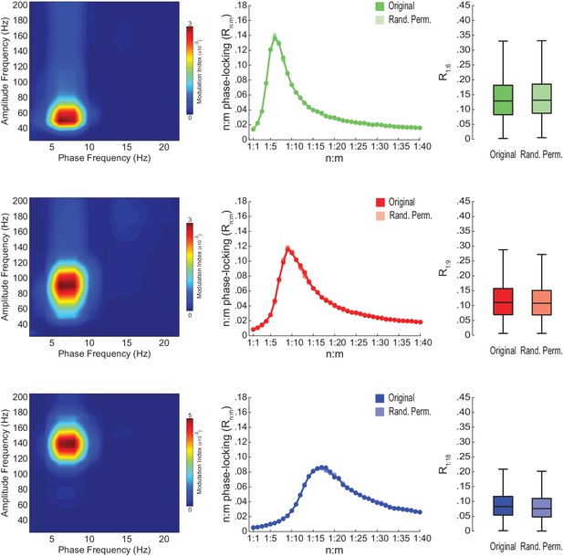
Lack of theta-gamma phase-phase coupling in independent components of gamma activity.
(Left) Average phase-amplitude comodulograms for three independent components (IC) that maximize coupling between theta phase and the amplitude of slow gamma (top row), middle gamma (middle row) and fast gamma (bottom row) oscillations (n = 4 animals). Each IC is a weighted sum of LFPs recorded in different hippocampal layers (see Schomburg et al., 2014). (Middle) n:m phase-locking levels for theta phase and the phase of ICs filtered at the gamma band maximally coupled to theta in the phase-amplitude comodulogram. (Right) Original and surrogate distributions of Rn:m values. Rn:m values were computed for 1 s long epochs (n = 4 animals); surrogate gamma phases were obtained by Random Permutation/Single Run.
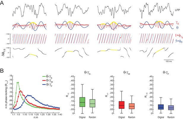
Lack of theta-gamma phase-phase coupling during transient gamma bursts.
(A) Examples of slow-gamma bursts. Top panels show raw LFPs, along with theta- (thick blue line) and slow gamma-filtered (thin red line) signals. The amplitude envelope of slow gamma is also shown (thick red line). The bottom rows show gamma and accelerated theta phases (m = 5), along with their instantaneous phase difference (). For each gamma sub-band, a ‘gamma burst’ was defined to occur when the gamma amplitude envelope was 2SD above the mean. In these examples, periods identified as slow-gamma bursts are marked with yellow in the amplitude envelope and phase difference time series. Notice variable across different burst events. (B) The left panel shows n:m phase-locking levels for theta phase and the phase of different gamma sub-bands (1 s epochs); for each gamma sub-band, Rn:m values were computed using only theta and gamma phases during periods of gamma bursts. The right panels show original and surrogate (Random Permutation/Single Run) distributions of Rn:m values (n = 4 animals).
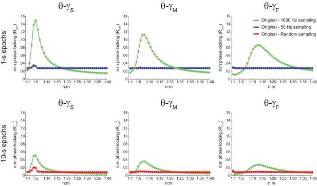
The bump in the Rn:m curve of hippocampal LFPs highly depends on analyzing contiguous phase time series data.
Average Rn:m curves computed for theta- and gamma-filtered hippocampal LFPs. The green curves were obtained using 1 s (top) or 10 s (bottom) continuous epochs of the phase time series, sampled at 1000 Hz (same analysis as in Figure 5A). The blue curves were obtained by analyzing 1000 data points subsampled from the phase time series at 20 Hz (i.e., 50 ms sampling period, longer than a gamma cycle). The red curves were obtained by analyzing 1000 (top) or 10000 (bottom) data points randomly sampled from the phase time series. These plots show that the prominent bump in the Rn:m curve of actual LFPs only occurs for continuously sampled data (1000 Hz sampling rate), and therefore probably reflects the ‘sinusoidality’ imposed by the filter (see also Figure 2—figure supplement 1). But notice that a small Rn:m bump remains for θ−γS (see Figure 10—figure supplement 2). Due to limitation of total epoch length, we could not perform the 20 Hz subsampling analysis for 10000 points, but notice that the blue and red curves coincide for 1000 points.
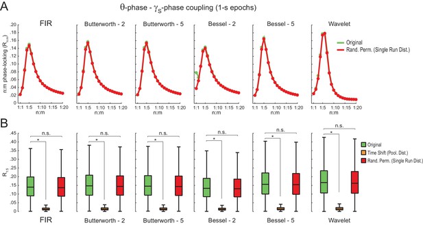
Different filter types give rise to similar results.
(A) Original (green) and surrogate (red) n:m phase-locking levels for actual hippocampal LFPs (same dataset as in Figure 5) filtered at theta and slow gamma (1 s epochs). Different rows show results for different types of filters. FIR corresponds to the same finite impulse response filter employed in all other figures. For the infinite impulse response filters (Butterworth and Bessel), the digit on the right denotes the filter order. Wavelet filtering was achieved by convolution with a complex Morlet wavelet with a center frequency of 7 Hz. (B) Original and surrogate distributions of R1:5 values. For each filter type, the original data is significantly higher than surrogate values obtained from pooled , but indistinguishable from single run surrogates. *p<0.01, n = 7 animals, Friedman’s test with Nemenyi post-hoc test.
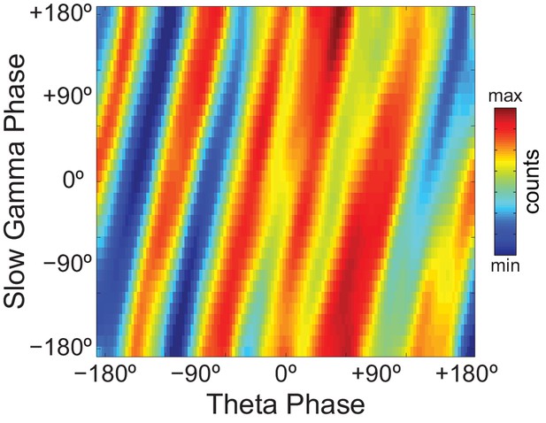
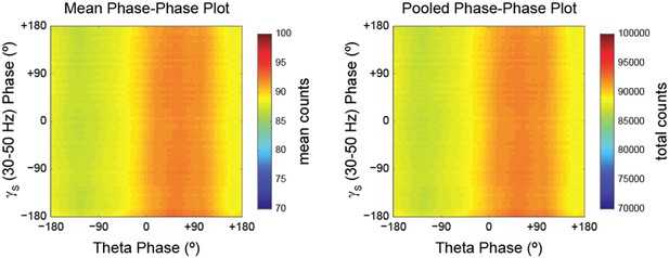
Phase-phase plots of hippocampal LFPs display diagonal stripes.
Phase-phase plot for theta and slow gamma (average over animals; n = 7 rats). Notice diagonal stripes suggesting phase-phase coupling.
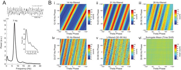
Phase–phase coupling between theta and gamma oscillations may be confounded by theta harmonics.
(A) Top, representative LFP epoch exhibiting prominent theta activity (~7 Hz) during REM sleep. Bottom, power spectral density. The inset shows power in dB scale. (B) Phase–phase plots for theta and LFP band-pass filtered at harmonic frequencies (14, 21, 28 and 35 Hz), computed using 20 min of concatenated REM sleep. Also shown are phase-phase plots for the conventional gamma band (30–90 Hz) and for the average over individual surrogate runs. Notice that the former mirrors the phase-phase plot of the fourth theta harmonics (35 Hz).
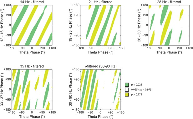
Histogram counts leading to diagonal stripes in phase-phase plots are statistically significant when compared to the distribution of surrogate counts.
Panels show the significance of the phase-phase plots in Figure 7 when compared to the mean and standard deviation of pooled surrogate counts.
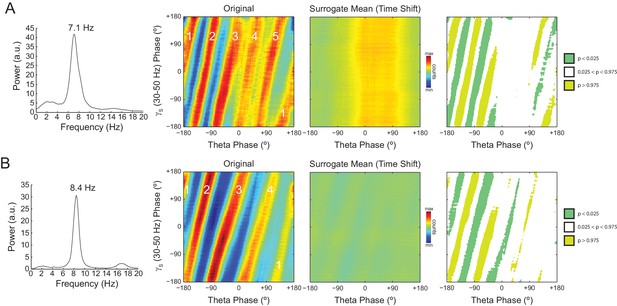
The number of stripes in phase-phase plots is determined by the frequency of the first theta harmonic within the filtered gamma range.
(A) Representative example in which theta has peak frequency of 7.1 Hz. The phase-phase plot between theta and slow gamma (30–50 Hz) exhibits five stripes, since the fourth theta harmonic (35.5 Hz) is the first to fall within 30 and 50 Hz. The rightmost panels show the average phase-phase plot computed over all time-shifted surrogate runs (n = 1000) and the significance of the original plot when compared to the mean and standard deviation over individual surrogate counts, respectively. (B) Example in which theta has peak frequency of 8.4 Hz and the phase-phase plot exhibits four stripes, which correspond to the third theta harmonic (33.6 Hz).
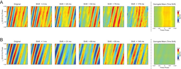
Individual time-shifted surrogate runs exhibit diagonal stripes in phase-phase plots.
(A) The middle panels show phase-phase plots for theta and slow gamma computed for different time shifts of the example epoch analyzed in Figure 8A. Notice diagonal stripes in individual surrogate runs. The left- and the rightmost panels show the original and average surrogate phase-phase plots, respectively (same panels as in Figure 8A). (B) Same as above, but for the example epoch analyzed in Figure 8B.
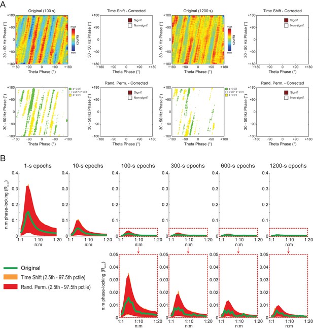
Phase-phase plots of white-noise signals display diagonal stripes.
(A) Representative phase-phase plots computed for white-noise signals. Notice the presence of diagonal stripes for both 100 s (left) and 1200 s (right) epochs. The colormaps underneath show the p-values of the original bin counts when compared to the mean and standard deviation over bin counts of single time-shifted surrogate runs. Also shown are significance maps after correcting for multiple comparisons (Holm-Bonferroni) using either time-shifted (top) or randomly permutated (bottom) surrogate runs. No bin count was considered statistically significant after the correction. (B) The top panels show original Rn:m curves (green) plotted along with Single Run distributions of Rn:m curves of time-shifted (orange) and randomly permutated (red) surrogates for different epoch lengths (shades denote the 2.5th–97.5th percentile interval; n = 2100 per distribution). The bottom panels show the same in a zoomed scale.
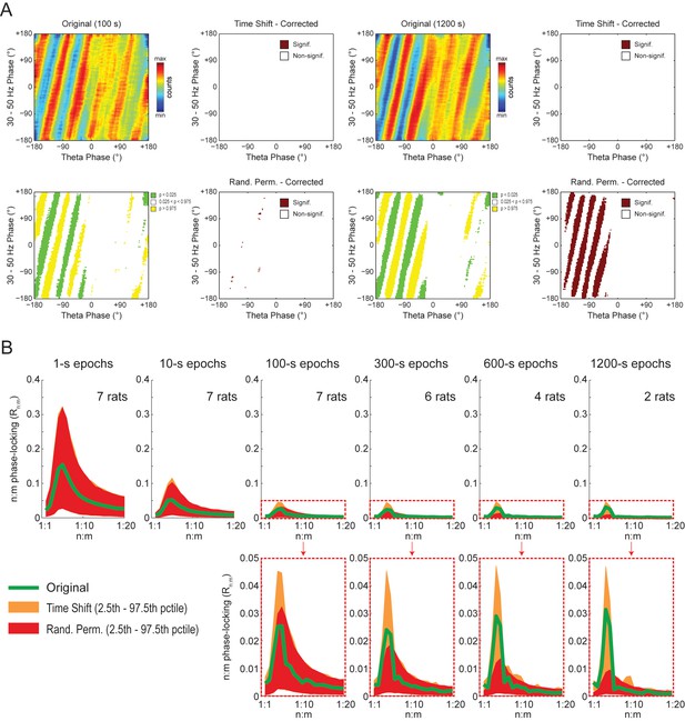
Weak but statistically significant n:m phase-locking can be detected when analyzing long LFP epochs (>100 s).
(A) Panels show the same as in Figure 9A but for a representative hippocampal LFP. Notice that several bin counts of the 1200 s epoch remain statistically significant after correction for multiple comparisons (Holm-Bonferroni) when compared to randomly permutated, but not time-shifted, surrogates (bottom right plot). (B) As in Figure 9B, but for actual LFPs (n = 300 samples per animal; the number of analyzed animals is stated in each panel). For the very long epochs, notice that the original Rn:m curve falls within the distribution of time-shifted surrogates but outside the distribution of randomly permutated ones.
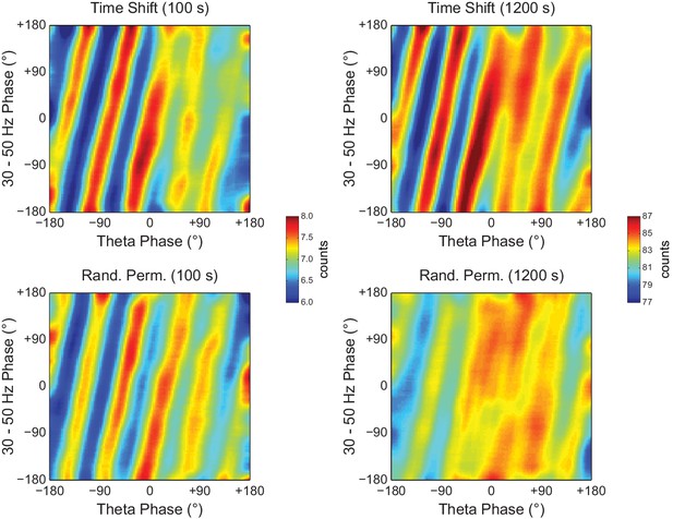
Random Permutation leads to less visible diagonal stripes than Time Shift in phase-phase plots of long LFP epochs.
Examples of phase-phase plots computed for single Time Shift (top) and Random Permutation (bottom) surrogate runs of 100 (left) and 1200 s (right) for the same hippocampal LFP as in Figure 10A. Notice that, for the longer LFP epoch, the randomly permutated surrogate exhibits less discernible stripes than the time-shifted one.
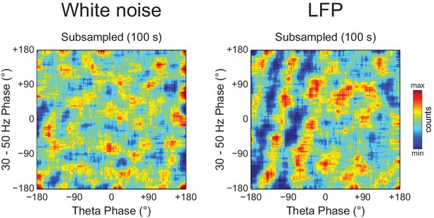
Diagonal stripes in phase-phase plots depend on analyzing contiguous phase time series data.
Phase-phase plots of a white noise (left) and an actual LFP (right) computed using 100 s of total data, but subsampled at 83.3 Hz (we used a subsampling period of 12 ms because the total data length of the actual LFP was 1200 s). Notice no diagonal stripes in the phase-phase plot of white noise, while some striped-like pattern persists for the actual LFP data.
