Dendritic trafficking faces physiologically critical speed-precision tradeoffs
- University of California, San Diego, United States
- Salk Institute for Biological Studies, United States
- Stanford University, United States
- University of Bristol, United Kingdom
- Brandeis University, United States
- University of Cambridge, United Kingdom
Figures
Figure 1 with 1 supplement
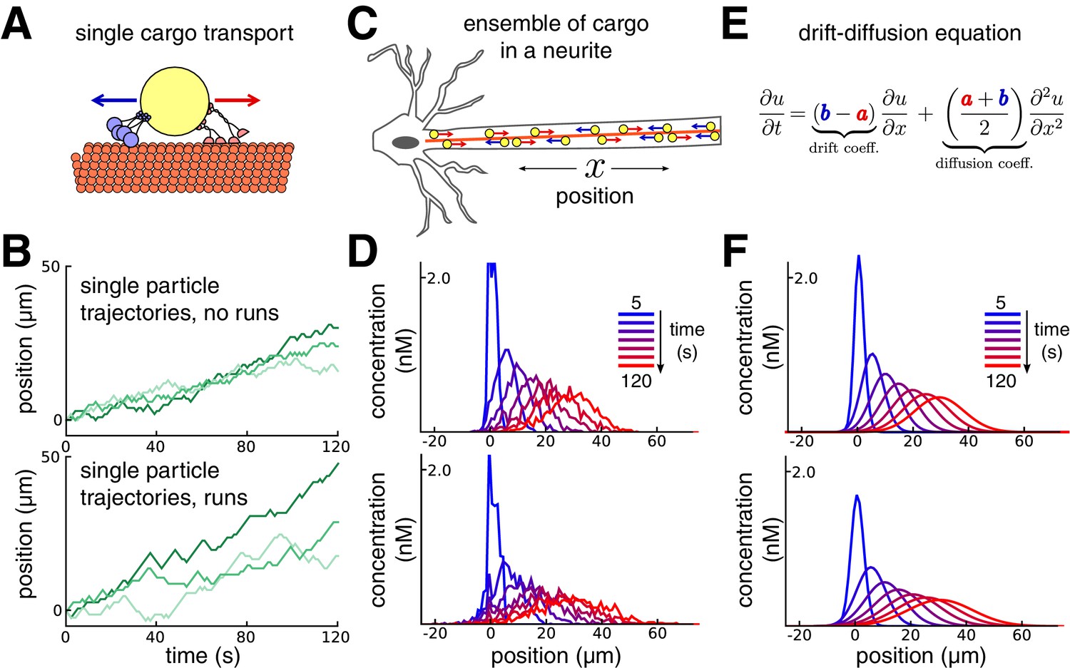
Constructing a coarse-grained model of intracellular transport.
(A) Cartoon of a single cargo particle on a microtubule attached to opposing motor proteins. (B) Three example biased random walks, representing the stochastic movements of individual cargoes. (Top panel) A simple random walk with each step independent of previous steps. (Bottom panel) Adding history-dependence to the biased random walk results in sustained unidirectional runs and stalls in movement. (C) Cartoon of a population of cargo particles being transported along the length of a neurite. (D) Concentration profile of a population of cargoes, simulated as 1000 independent random walks along a cable/neurite. (Top panel) simulations without runs. (Bottom panel) Simulations with runs. (E) In the limit of many individual cargo particles, the concentration of particles is described by a drift diffusion model whose parameters, and , map onto the mass action model (Equation 1). (F) The mass-action model provides a good fit to the simulations of bulk cargo movement in (D). (Top panel) Fitted trafficking rates for the model with no runs were a ≈ 0.42 s−1, b ≈ 0.17 s−1. (Bottom panel) Fitting the model with runs gives a ≈ 0.79 s−1, b ≈ 0.54 s−1.
Figure 1—figure supplement 1
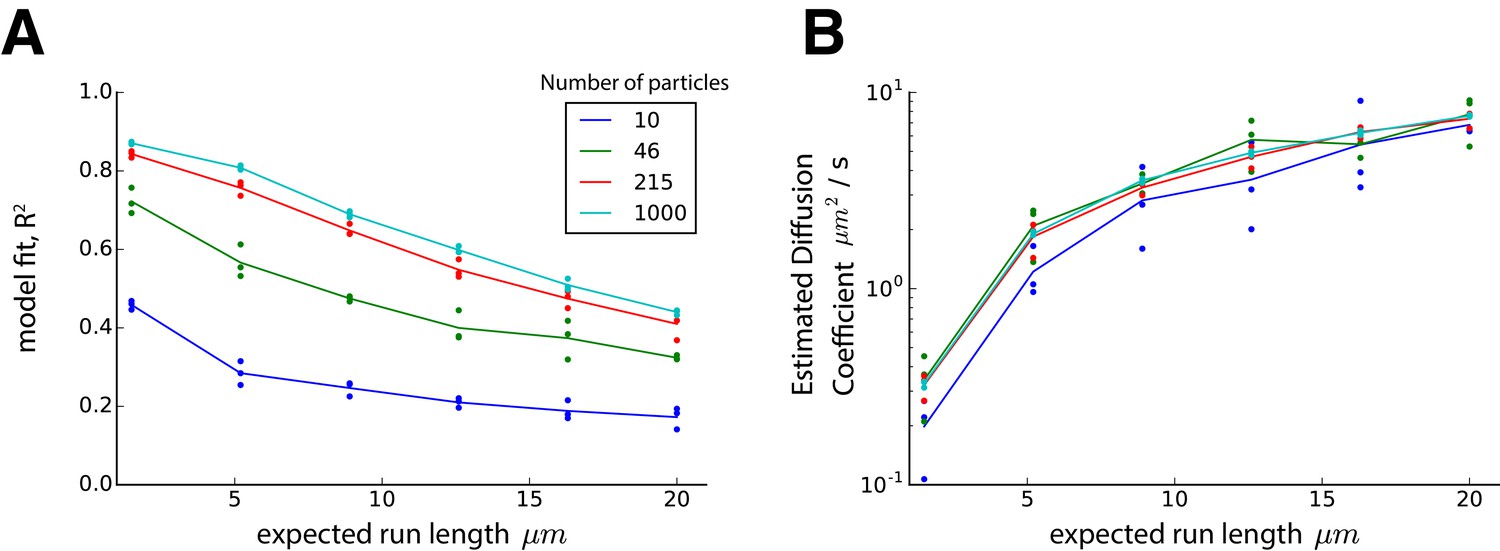
The effect of cargo run length on mass-action model fit and diffusion coefficient.
The model of stochastic particle movement (Equation 7, Materials and methods) was simulated with equal transition probabilities () for various values of and particle numbers in an infinite cable with 1 µm compartments and 1 s time steps. The expected run length is given by the mean of a negative binomial distribution. For each simulation, a mass-action approximation was fit by matching the first two moments of the cargo distribution, as described in the Materials and methods. In both panels, dots represent simulated triplicates, and lines denote the average outcome with colors denoting the simulated ensemble size (see legend). (A) The mass-action model (Equation 1, Results) provides a reasonably accurate fit after 100 s of simulation with moderately long run lengths and low particle numbers. The fit improves for longer simulations and larger particle numbers, since the cargo distribution is better approximated by a normal distribution under these conditions due to the central limit theorem. The coefficient of determination, , reflects the proportion of explained variance by the mass-action model (equivalent to a Gaussian fit to the concentration profile). (B) The estimated diffusion coefficient of the mass-action model (i.e. the variance of the Gaussian fit in panel A) increases as expected run length increases.
Figure 2 with 1 supplement
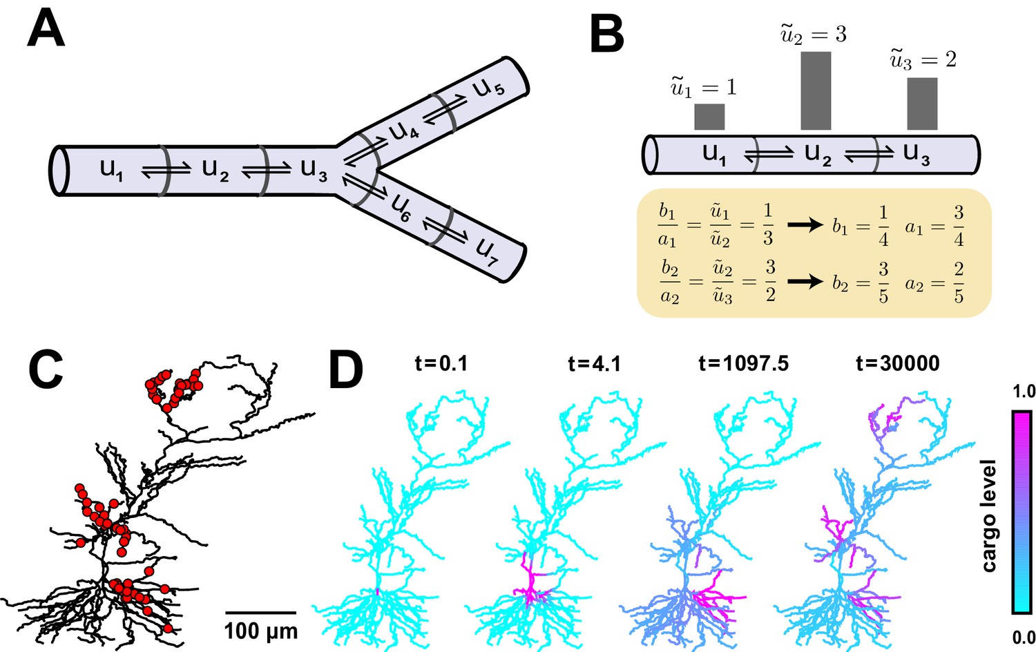
Local trafficking rates determine the spatial distribution of biomolecules by a simple kinetic relationship.
(A) The mass action transport model for a simple branched morphology. (B) Demonstration of how trafficking rates can be tuned to distribute cargo to match a demand signal. Each pair of rate constants (, ) was constrained to sum to one. This constraint, combined with the condition in Equation (4), specifies a unique solution to achieve the demand profile. (C) A model of a CA1 pyramidal cell with 742 compartments adapted from (Migliore and Migliore, 2012). Spatial cargo demand was set proportional to the average membrane potential due to excitatory synaptic input applied at the locations marked by red dots. (D) Convergence of the cargo concentration in the CA1 model over time, (arbitrary units).
Figure 2—figure supplement 1
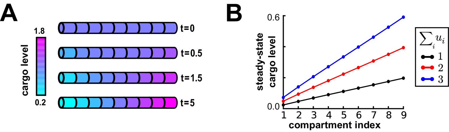
Equation 4 specifies the relative distribution of cargo, changing the total amount of cargo scales this distribution.
(A) Inspired by ion channel expression gradients observed in hippocampal cells (Hoffman et al., 1997; Magee, 1998), we produced a linear gradient in cargo distribution in an unbranched cable. By Equation 4, the trafficking rate constants satisfy (where indexes on increasing distance to the soma). Starting from a uniform distribution of cargo in the cable ( a.u.), the desired linear profile emerges over time. (B) Changing the amount of cargo in the cable (the sum of across all compartments, see legend) does not disrupt the steady-state linear expression profile, but scales its slope.
Figure 3
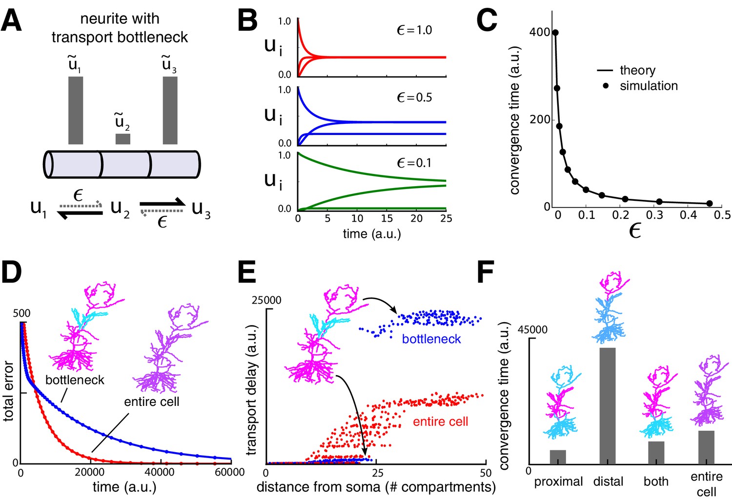
Transport bottlenecks caused by cargo demand profiles.
(A) A three-compartment transport model, with the middle compartment generating a bottleneck. The vertical bars represent the desired steady-state concentration of cargo in each compartment. The rate of transport into the middle compartment is small (, dashed arrows) relative to transport out of the middle compartment. (B) Convergence of cargo concentration in all compartments of model in (A) for decreasing relative bottleneck flow rate, . (C) Simulations (black dots) confirm that the time to convergence is given by the smallest non-zero eigenvalue of the system (solid curve). (D) Convergence to a uniform demand distribution (red line) is faster than a target distribution containing a bottleneck (blue line) in the CA1 model. Total error is the sum of the absolute difference in concentration from demand ( norm). Neuron morphologies are color-coded according to steady state cargo concentration. (E) Transport delay for each compartment in the CA1 model (time to accumulate 0.001 units of cargo). (F) Bar plot comparison of the convergence times for different spatial demand distributions in the CA1 model (steady-state indicated in color plots). The timescale for all simulations in the CA1 model was normalized by setting for each compartment.
Figure 4

Multiple strategies for transport with trafficking and cargo detachment controlled by local signals.
(A) Schematic of microtubular transport model with irreversible detachment in a branched morphology. (B) Multiple strategies for trafficking cargo to match local demand (demand = ). (Top) The demand-dependent trafficking mechanism (DDT). When the timescale of detachment is sufficiently slow, the distribution of cargo on the microtubules approaches a quasi-steady-state that matches spatially. This distribution is then transformed into the distribution of detached cargo, . (Bottom) The demand dependent detachment (DDD) mechanism. Uniform trafficking spreads cargo throughout the dendrites, then demand is matched by slowly detaching cargo according to the local demand signal. An entire family of mixed strategies is achieved by interpolating between DDT and DDD. (C–E) Quasi-steady-state distribution of cargo on the microtubules (, red) and steady-state distribution of detached cargo (, blue), shown with a demand profile (, black) for the various strategies diagrammed in panel B. The demand profile is shown spatially in the color-coded CA1 neuron in the right of panel C. Detached cargo matches demand in all cases.
Figure 5
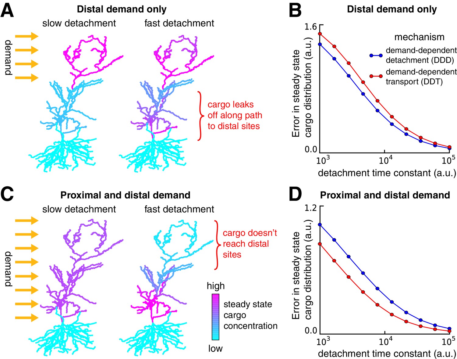
Tradeoffs in the performance of trafficking strategies depends on the spatial pattern of demand.
(A) Delivery of cargo to the distal dendrites with slow (left) and fast detachment rates (right) in a reconstructed CA1 neuron. The achieved pattern does not match the target distribution when detachment is fast, since some cargo is erroneously delivered to proximal sites. (B) Tradeoff curves between spatial delivery error and convergence rate for the DDT (red line, see Figure 4C) and DDD (blue line, see Figure 4D) trafficking strategies. (C–D) Same as (A–B) but with uniform demand throughout proximal and distal locations. The timescale of all simulations was set by imposing the constraint that for each compartment, to permit comparison.
Figure 6 with 1 supplement
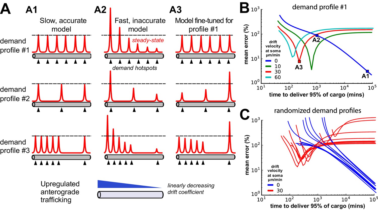
Tuning the DDD model for speed and specificity results in sensitivity to the target spatial distribution of cargo.
(A) Cargo begins on the left end of an unbranched cable to be distributed equally amongst several demand ‘hotspots’. Steady-state cargo profiles (red) are shown for three different models (A1, A2, A3) and three different spatial patterns of demand (rows). The bottom panel shows an upregulated anterograde trafficking profile introduced to reduce delivery time in A3; soma is at the leftmost point of the cable. (A1) A model with sufficiently slow detachment achieves near-perfect cargo delivery for all demand patterns. (A2) Making detachment faster produces quicker convergence, but errors in cargo distribution. (A3) Transport rate constants, and , were tuned to optimize the distribution of cargo for the first demand pattern (top row); detachment rate constants were the same as in model A2. (B) Tradeoff curves between non-specificity and convergence rate for six evenly spaced demand hotspots (the top row of panel A). Tradeoff curves are shown for the DDD model (blue line) as well as models that combine DDD with the upregulated anterograde trafficking profile (as in A, bottom panel). Marked points denote where models A1, A2, A3 sit on these tradeoff curves. (C) Tradeoff curves for randomized demand patterns (six uniformly placed hotspots). Ten simulations are shown for the DDD model with (red) and without (blue) anterograde trafficking upregulation.
Figure 6—figure supplement 1
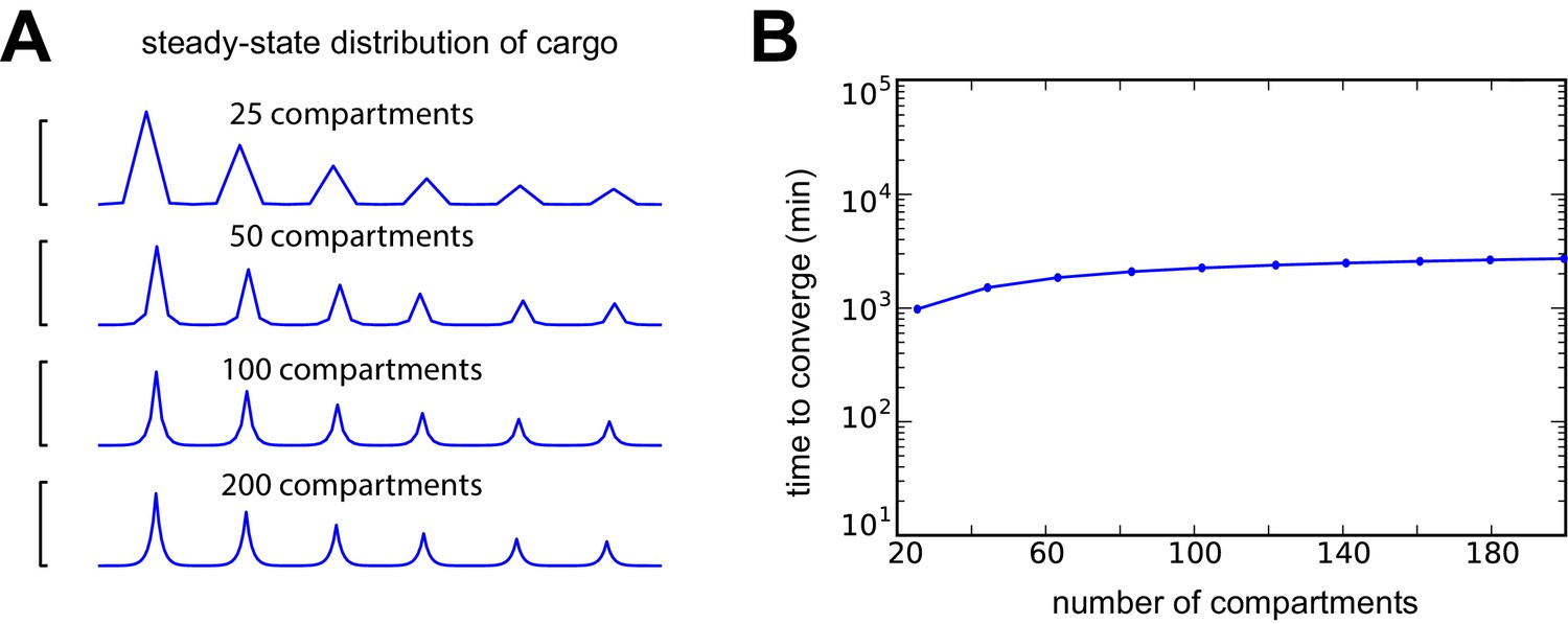
Changing compartment size over an order of magnitude leads to insignificant changes in model behavior when trafficking rates are appropriately scaled (i.e. and are inversely scaled to the squared compartment length; the diffusion coefficient converges to 10 μm2 s−1 as the compartment size shrinks to zero).
(A) A DDD model with six evenly spaced demand hotspots along a 800 µm cable and a fixed detachment rate constant of 5 × 10⁻⁴ s−1 converges to the same qualitative distribution of cargo at steady-state when the number of compartments is varied. (B) Number of minutes to deliver 90% of cargo as a function of compartment number. Despite order-of-magnitude changes in compartment size, the convergence time changes much less.
Figure 7
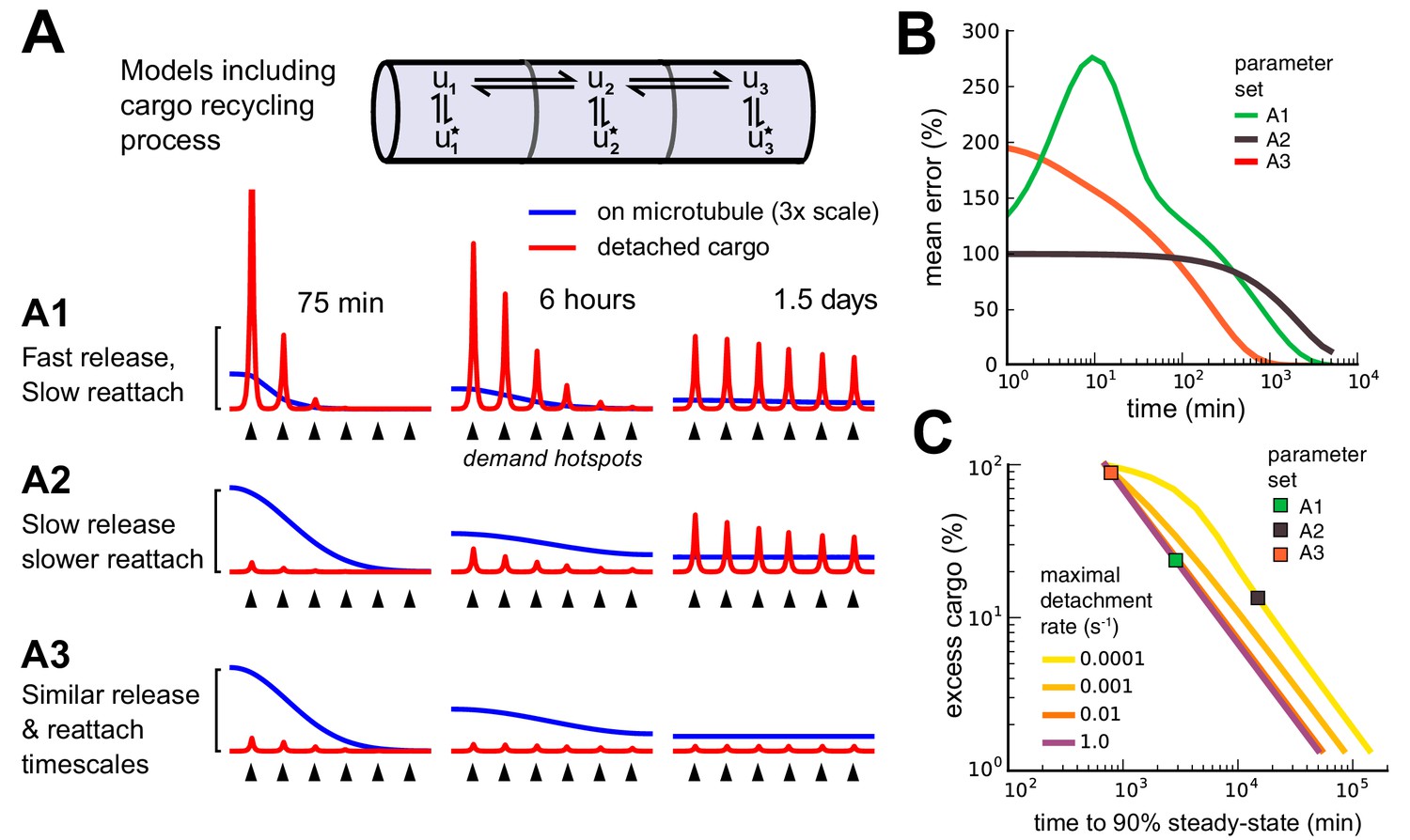
Adding a mechanism for cargo reattachment produces a further tradeoff between rate of delivery and excess cargo.
(A) Simulations of three models (A1, A2, A3) with cargo recycling. As in Figure 6, cargo is distributed to six demand hotspots (black arrows). The distributions of cargo on the microtubules (, blue) and detached cargo (, red) are shown at three times points for each model. (B) Mean percent error in the distribution of detached cargo as a function of time for the three models in panel A. (C) Tradeoff curves between excess cargo and time to convergence to steady-state (within 10% mean error across compartments) for fixed cargo detachment timescales (line color). For all detachment timescales, varying the reattachment timescale produced a tradeoff between excess cargo (fast reattachment) and slow convergence (slow reattachment). Colored squares denote the position of the three models in panel A.
Figure 8
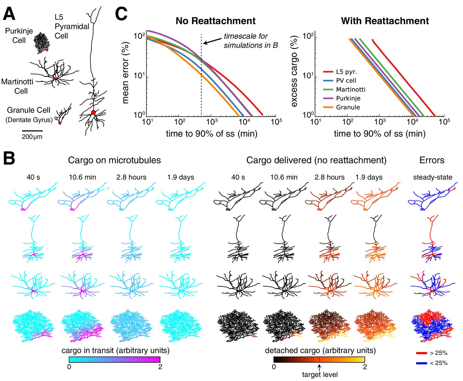
Effect of morphology on trafficking tradeoffs.
(A) Representative morphologies from four neuron types, drawn to scale. The red dot denotes the position of the soma (not to scale). (B) Distribution of cargo on the microtubles () and delivered cargo () at four time points for sushi-belt model with irreversible detachment. Cargo originated in the soma and was transported to a uniform distribution (all , normalized to a diffusion coefficient of 10 μm2 s-1); the detachment rate was spatially uniform and equal to 8 × 10⁻⁵ s−1. (C) Tradeoff curves for achieving a uniform distribution of cargo in realistic morphologies (PV cell = parvalbumin interneuron, morphology not shown). The sushi-belt model without reattachment (as introduced in Figure 4) suffers a tradeoff in speed and accuracy, while including reattachment (as in Figure 7) produces a similar tradeoff between speed and excess ‘left-over’ cargo. An optimistic diffusion coefficient of 10 μm2 s−1 was used in both cases. For simulations with reattachment, the detachment rate () was set equal to trafficking rates () for a one micron compartment. The dashed line denotes the convergence timescale for all simulations in panel B.
Videos
Video 1
Distribution of trafficked cargo over logarithmically spaced time points in a CA1 pyramidal cell model adapted from (Migliore and Migliore, 2012).
Cargo was trafficked according to Equation 4 to match a demand signal established by stimulated synaptic inputs (see Figure 2C). Time and cargo concentrations are reported in arbitrary units.
Video 2
A model with slow detachment rate accurately distributes cargo to six demand hotspots in an unbranched cable.
The spatial distribution of detached cargo (bottom subplot) and cargo on the microtubules (top subplot) are shown over logarithmically spaced timepoints. Compare to Figure 6A1 (top row).
Video 3
A model with a fast detachment rate misallocates cargo to six demand hotspots in an unbranched cable.
The spatial distribution of detached cargo (bottom subplot) and cargo on the microtubules (top subplot) are shown over logarithmically spaced timepoints. Proximal demand hotspots receive too much cargo, while distal regions receive too little. Compare to Figure 6A2 (top row).
Video 4
Fine-tuning the trafficking rates in a model with fast detachment produces fast and accurate deliver of cargo to six demand hotspots in an unbranched cable.
The spatial distribution of detached cargo (bottom subplot) and cargo on the microtubules (top subplot) are shown over logarithmically spaced timepoints. Compare to Figure 6A3 (top row).
Video 5
The model fine-tuned for fast and accurate deliver of cargo to six demand hotspots misallocates cargo to three demand hotspots.
The spatial distribution of detached cargo (bottom subplot) and cargo on the microtubules (top subplot) are shown over logarithmically spaced timepoints. Compare to Figure 6A3 (middle row).
Download links
A two-part list of links to download the article, or parts of the article, in various formats.
Downloads (link to download the article as PDF)
Open citations (links to open the citations from this article in various online reference manager services)
Cite this article (links to download the citations from this article in formats compatible with various reference manager tools)
Dendritic trafficking faces physiologically critical speed-precision tradeoffs
eLife 5:e20556.
https://doi.org/10.7554/eLife.20556


