Biologically plausible learning in recurrent neural networks reproduces neural dynamics observed during cognitive tasks
- The Neurosciences Institute, United States
Figures
Figure 1
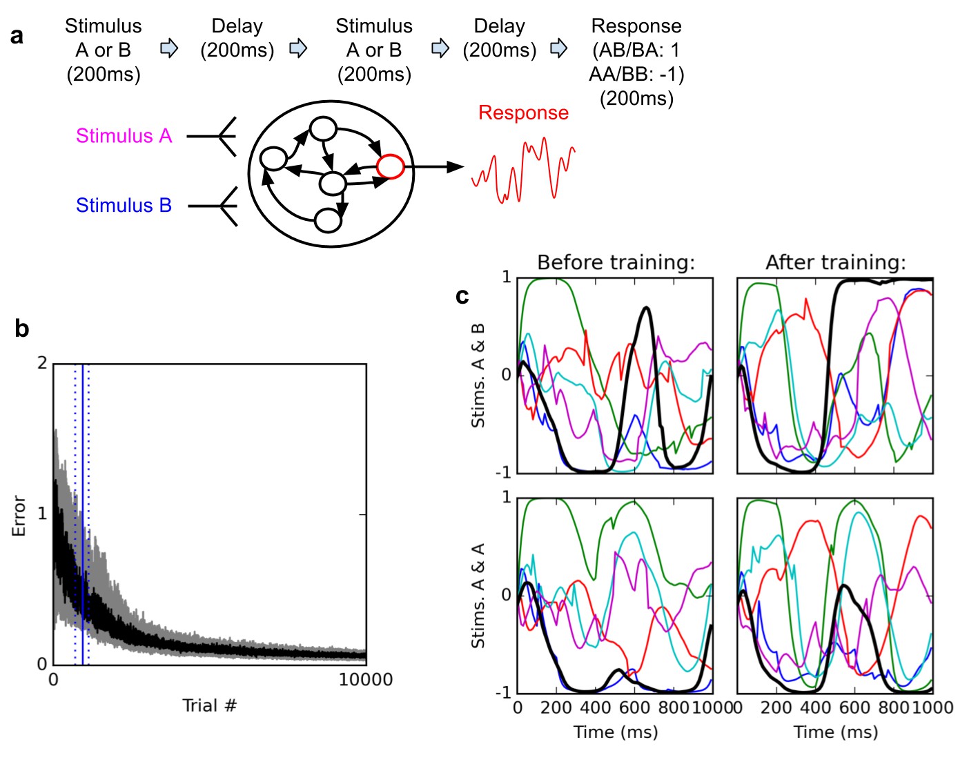
Delayed nonmatch-to-sample task.
(A) (top): task description. The network is exposed to two successive stimuli, with an intervening delay. The task is to produce output −1 if the two stimuli were identical (AA or BB), or 1 if they were different (AB or BA); the output of the network is simply the activity of one arbitrarily chosen ‘output’ neuron, averaged over the last 200 ms of the trial. (B) (bottom left): time course of trial error (mean absolute difference between output neuron response and correct response over the last 200 ms of each trial) during learning over 10000 trials (dark curve: median over 20 runs; gray area: inter-quartile range). The solid vertical line indicates the median number of trials needed to reach the criterion of 95% ‘correct’ trials (trial error <1) over 100 successive trials (843 trials); dotted vertical lines indicate the inter-quartile range (692–1125 trials). Performance (i.e., magnitude of the response error) continues to improve after reaching criterion and reaches a low, stable residual asymptote. ( (bottom right): Activities of 6 different neurons, including the output neuron (thick black line), for two stimulus combinations, before training (left) and after training (right). Note that neural traces remain highly dynamical even after training.
Figure 2
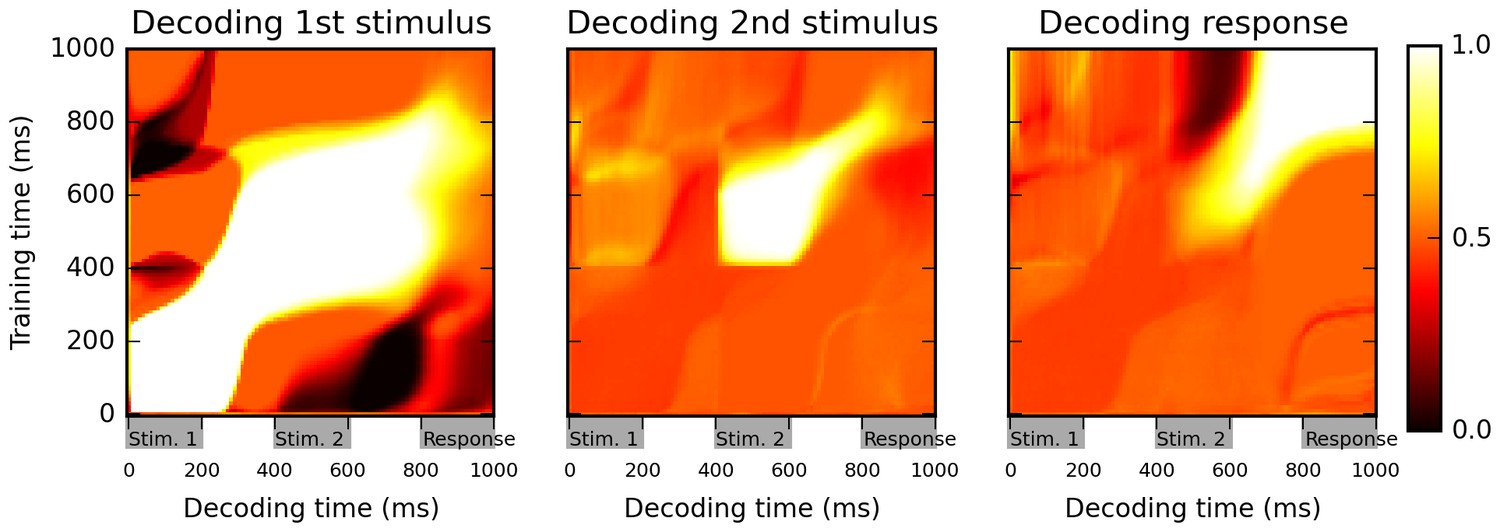
Cross-temporal classification performance reveals dynamic coding.
Cross-temporal classification of 1st stimulus identity (left panel), 2nd stimulus identity (middle panel) and network response (right panel). Row i and column j of each matrix indicates the accuracy of a classifier, trained on population activity data at time i, in guessing a specific task feature using population activity data at time j (training and decoding data are always separate). While the network reliably encodes information about stimulus identity right until the onset of the response period (as shown by high accuracy values along the diagonal in left and middle panel), this information is stored with a highly dynamic encoding (as shown by low cross-classification accuracy across successive periods, i.e., ‘bottlenecks’ with high accuracy on the diagonal but low accuracy away from the diagonal). Note that in both left and middle panels, stimulus identity information decreases greatly at the onset of the response period, reflecting a shift to a from stimulus-specific to response-specific encoding (see also Figure 3).
Figure 3

Multi-dimensional scaling plots of population activity reflect shifting encodings of task-relevant information.
Population response vectors at various points in time (color-coded by stimulus combination) are projected in two dimensions while preserving distances between data points as much as possible, using multi-dimensional scaling. At the end of the first stimulus presentation (200 ms), population states are firmly separated by first stimulus identity, as expected. After the second stimulus presentation (600 ms), all four possible stimulus combinations lead to clearly separate population activity states. However, population states corresponding to different responses start to cluster together at the onset of the response period (800 ms). Late in the response period (1000 ms), population trajectories corresponding to the same response (AA and BB, or BA and AB) have largely merged together, reflecting a shift from stimulus-specific to response-specific representation and a successful ‘routing’ of individual stimulus-specific states to the adequate response-specific state.
Figure 4
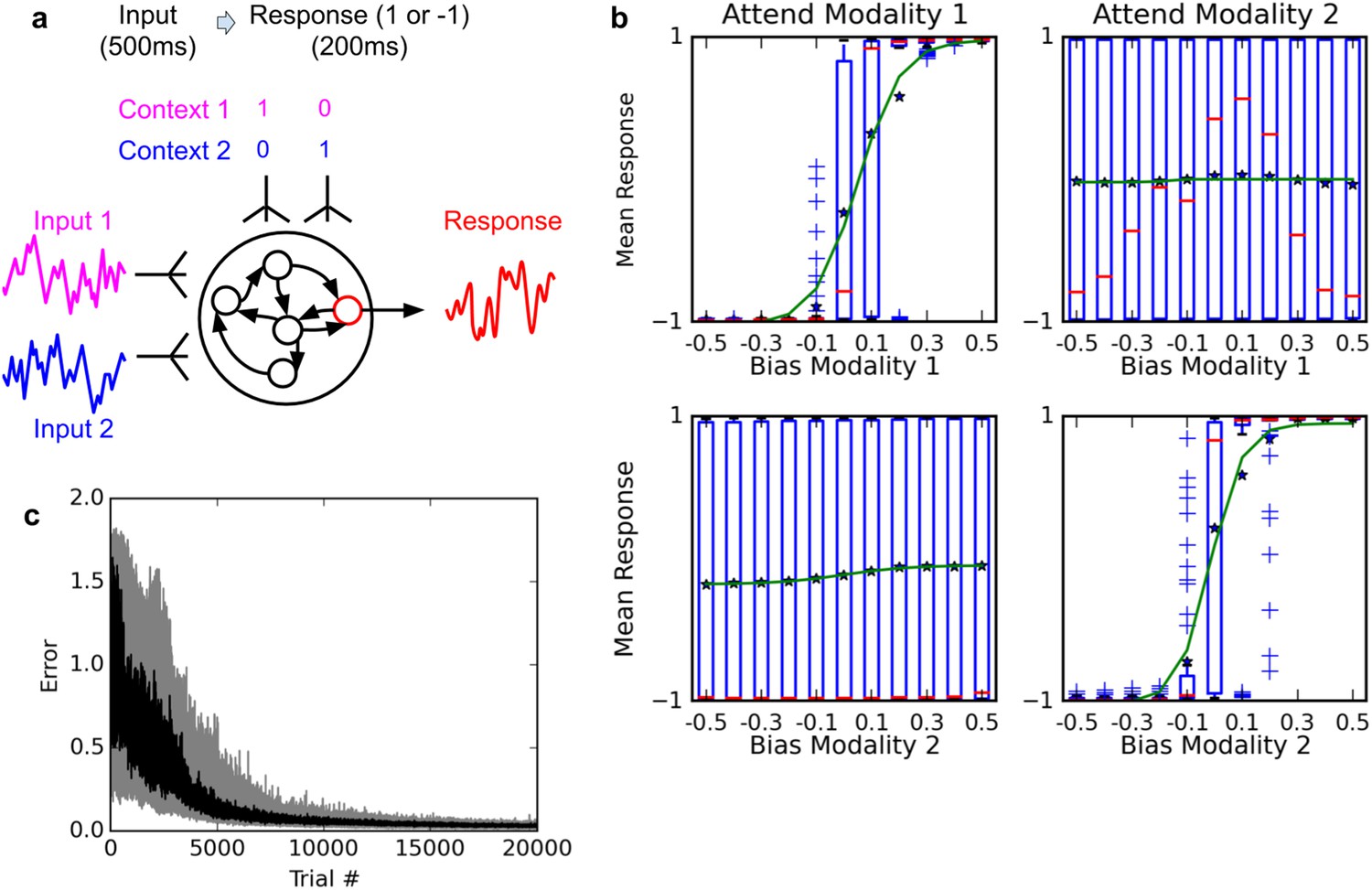
Selective integration task.
(A) (top left): task description. The network receives two noisy inputs, simulating sensory information coming from two different modalities, as well as two ‘context’ inputs to indicate which of the two sensory inputs must be attended. The task is to produce output 1 if the cued input has a positive mean, and −1 if the cued input has negative mean; this task requires both selective attention and temporal integration of the attended input. (B) (top right): Psychometric curves of network responses. Responses are segregated according to the value of the relevant modality bias, and shown as box-plots: blue boxes indicate the inter-quartile range, with data points outside the box showing as blue crosses; red bars indicate medians, and dark stars indicate means; green curves are sigmoid fits to the means. Top-left panel: Responses when context requires attending to modality 1, sorted by the bias of modality 1 inputs. The network response correctly tracks the overall bias of modality 1 inputs. Bottom-left panel: same data, but sorted by modality 2 bias. Network response is mostly unaffected by modality 2 bias, as expected since the network is required to attend to modality 1 only. Right panels: network responses when the context requires attending to modality 2. Again, the network correctly identifies the direction of the relevant modality while mostly ignoring the irrelevant modality. (C) (Bottom): Median and inter-quartile range of trial error (mean absolute difference between output and correct response over the last 200 ms of the trial) over 20 runs of 20000 trials each.
Figure 5

Orthogonal decoding of population activities.
Population response patterns are averaged at each point in time, separately by context (i.e. relevant modality), final choice of the trial, and the bias of modality 1 (top) or 2 (bottom). For each combination of relevant modality and averaging modality, these averaged patterns over time result in different trajectories (one per value of the averaging modality, ranging from −0.25 (bright red) to 0.25 (bright green)). We project these trajectories over dimensions indicating how reliably the network encodes modality 1 value, modality 2 value, and final choice. In all graphs, the x axis is the dimension that reflects current encoding of final choice; the y axis is the dimension that reflects current encoding of the grouping modality (i.e. the one used for averaging). Only correct trials are used (thus top-left and bottom-right panels only have 10 trajectories, since correct trials with positive bias in the relevant modality cannot lead to a negative choice, and vice versa). The trajectories reveal that the network encodes both the relevant and the irrelevant modality, though only the relevant one is linked to the final choice. See text for details.
Figure 6
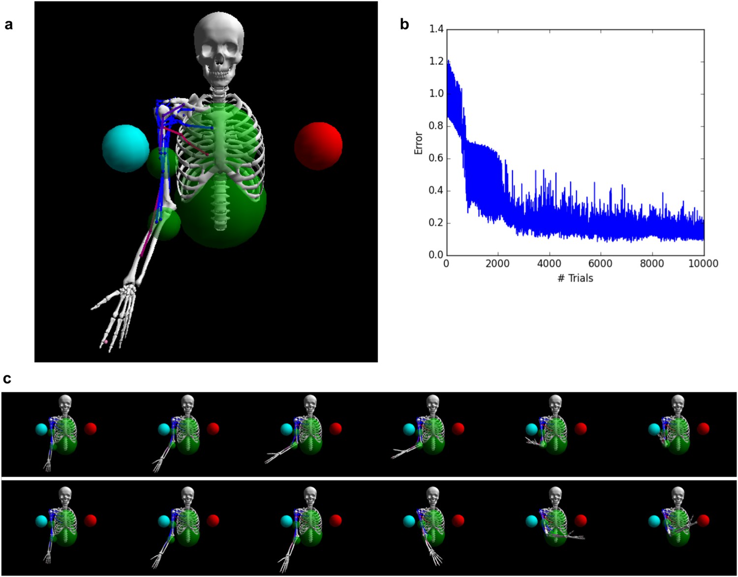
Controlling a biophysical model of the human arm.
(A) (top left): A model of the human upper skeleton with 4 degrees of freedom (shoulder and elbow joints), actuated by 16 muscles at the shoulder, chest and arm (colored strings represent muscles; blue indicates low activation, red indicates high activation). The task is to reach either of two target balls (blue or red), depending on a context input. (B) (top right): During training, the error (measured by the distance between tip of hand and target ball at the end of each trial) improves immediately and reaches a low residual plateau after about 3000 trials. (C) (bottom): frame-by-frame illustrations of a right-target trial (top row) and a left-target trial (bottom row), after training.
Figure 7
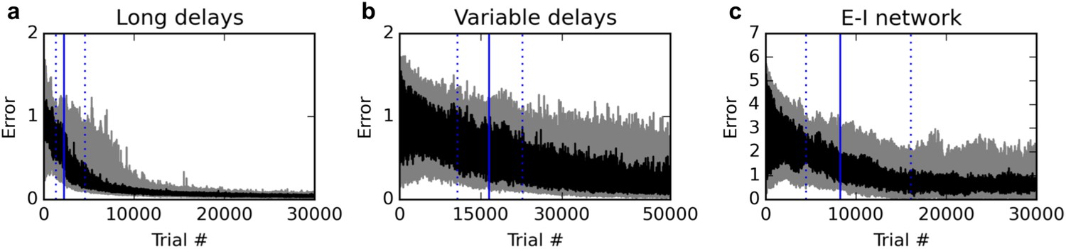
Additional experiments.
Panels show learning curves for the delayed nonmatch-to-sample task, modified in three ways. (A) (left): long 1000 ms delays. (B) (middle): variable inter-stimulus interval, randomly chosen from 300 to 800 ms. (C) (right): Networks with nonnegative neural responses and separate excitatory and inhibitory neurons (in accordance with Dale’s law). Conventions are as in Figure 1: dark lines indicate median over 20 runs, while gray shaded area indicates the inter-quartile range. See text for details.
Figure 8
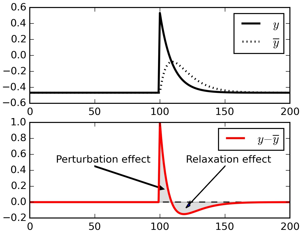
Relaxation effects.
When a perturbation is applied to signal, subtracting a running average initially extracts the perturbation, but then introduces opposite-sign terms as the running average relaxes to the signal.
Figure 9
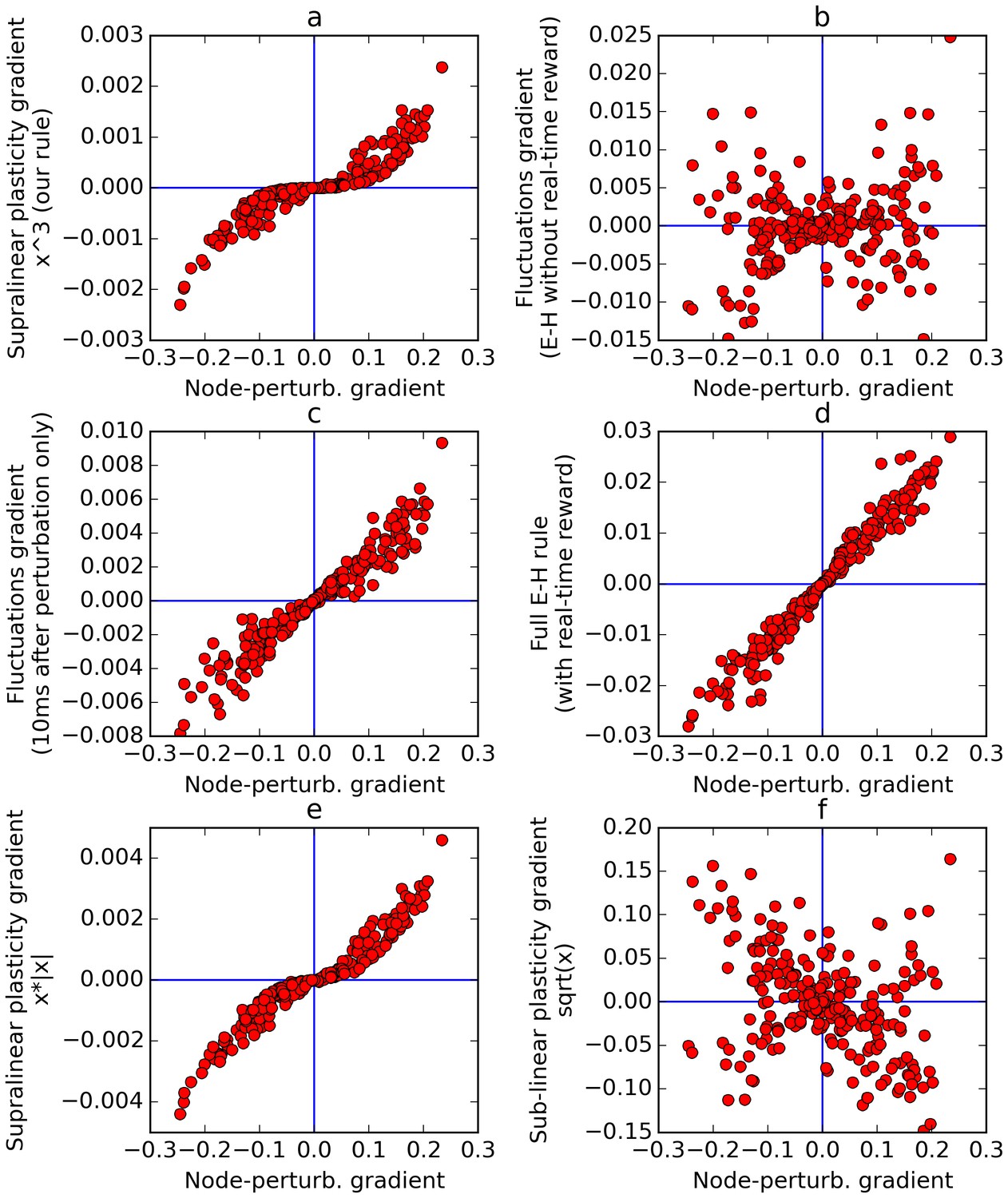
Comparison of error gradients.
A recurrent network is repeatedly exposed to randomly-chosen, time-constant inputs, and must learn to determine whether the inputs have positive sum. We compute the learning gradients over the weights according to various methods, for many trials, based on a single perturbation at a fixed time in each trial. In all four panels, the x-axis indicates the gradient computed by node-perturbation, used as a ground truth. Panel a: the weight modifications produced by node-perturbation align remarkably with the rule described in this paper. Panel b: gradients computed by using raw fluctuations of output about a running average, without supralinear amplification, are essentially random. Panel c: if we restrict the plasticity computations to the first 10 ms after perturbation, the correct gradients are recovered (using only 1 ms would be identical to panel a), confirming that post-perturbation effects are responsible. Panel d: The full E-H rule, with real-time reward signal, also recovers the node-perturbation gradients. Panel e: Using a different supralinear function (signed square rather than cubic) produces largely similar results to Panel a. Panel f: By contrast, a sublinear function (square root) results in largely random gradients.
Download links
A two-part list of links to download the article, or parts of the article, in various formats.
Downloads (link to download the article as PDF)
Open citations (links to open the citations from this article in various online reference manager services)
Cite this article (links to download the citations from this article in formats compatible with various reference manager tools)
Biologically plausible learning in recurrent neural networks reproduces neural dynamics observed during cognitive tasks
eLife 6:e20899.
https://doi.org/10.7554/eLife.20899


