Figures and data in Dynamic range adaptation in primary motor cortical populations | eLife

Figures

7 figures

Figures

Figure 1

Download asset Open asset

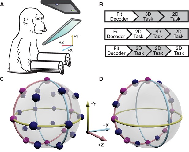
Experimental setup.

(A) The monkey controlled a computer cursor on a stereoscopic monitor viewed through a mirror, using neural signals. (B) Each recording session began with a brief calibration session to build the decoder. The decoder was used for a block of 3D trials (between 9 and 13 trials per target), followed by a block of 2D trials (between 15 and 27 trials per target). In some sessions, an additional block of 2D trials would proceed the blocks of 3D and 2D trials, or an additional block of 3D trails would follow the blocks of 3D and 2D trials. We focused our analyses on the first block of 3D trials and the block of 2D trials immediately following it (the gray boxes). In the supplementary materials, we demonstrate that our findings are invariant to the order of the blocks of trials. (C) Locations of the 26 targets in the 3D context. (D) Locations of the 16 targets in the 2D context. The eight targets that were common to the 2D and 3D contexts are shown in pink. The red, yellow, and light blue hoops represent the xy-plane, xz-plane, and yz-plane, respectively. Data of the target locations are available in Figure 1—source data 1.

https://doi.org/10.7554/eLife.21409.003

Figure 1—source data 1 Target location dataset.: https://doi.org/10.7554/eLife.21409.004
Download elife-21409-fig1-data1-v1.zip

Figure 2 with 5 supplements

Download asset Open asset

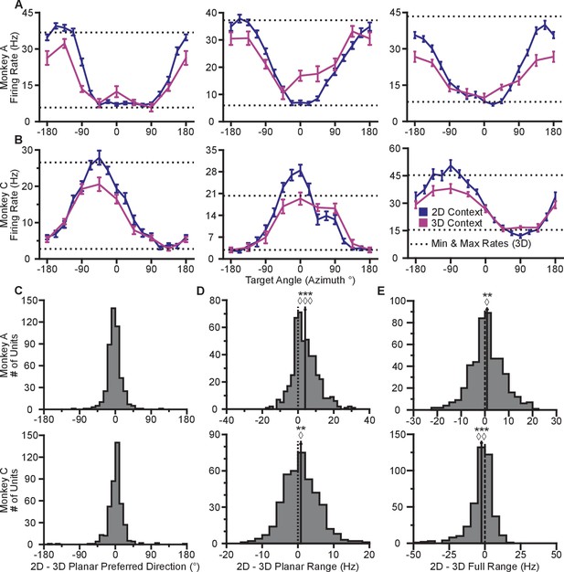
Tuning differences between the 2D and 3D contexts.

(A, B) Selected tuning curves for the targets in the xy-plane during the 3D (pink) and 2D (dark blue) contexts from Monkey A (panel A) and Monkey C (panel B). Firing rates show the mean $\pm$ SE for each target. There were 10 trials per target in the 3D task for all units shown with the exception of the last unit in (B) where there were 12 trials per target. There were 15 trials per target in the 2D task for all units shown with the exception of the first two units in (panel A) where there were 27 trials per target. The dashed horizontal lines show the minimum and maximum target-averaged firing rates for all 26 targets in the 3D context. (C) Changes in azimuthal preferred direction for Monkey A (top) and Monkey C (bottom). Firing rates were used to fit log-linear tuning models independently for the 2D and 3D contexts to calculate the preferred directions of the units. The preferred direction from the 2D context was compared to the $x$ and $y$ -components of the preferred direction from the 3D context to calculate the change in the azimuthal preferred direction. The changes are insignificant under the Moore test of paired samples of angles for both Monkey A ( $R^{'} = 0.817$ , $n = 471$ , $P > 0.1$ ) and Monkey C ( $R^{'} = 0.887$ , $n = 409$ , $P > 0.05$ ). (D) Histograms of the differences in tuning ranges for the set of eight identical targets between the 2D and 3D contexts for Monkey A (top) and Monkey C (bottom). For both panels: solid vertical lines, means of distributions; solid horizontal lines, mean $\pm$ SE; dashed vertical lines, point of equality between the two tuning ranges. In both subjects, the 2D planar dynamic range was larger than the 3D planar dynamic range (Monkey A: *** $P ≪ 10^{- 20}$ , Wilcoxon signed-rank test, $W = 88059$ , $◊ ◊ ◊ P < 10^{- 18}$ , sign test, $S = 334$ , $n = 471$ units; Monkey C: ** $P = 0.0032$ , $W = 48975$ , $◊ P = 0.0134$ , $S = 230$ , $n = 409$ units). (E) Histograms of the differences in tuning ranges for the full set of targets between the 2D and 3D contexts for Monkey A (top) and Monkey C (bottom). The full tuning range was greater in the 2D context for Monkey A (** $P = 0.0081$ , $W = 63402$ , $◊ P = 0.0426$ , $S = 258$ , $n = 471$ ) and in the 3D context for Monkey C (*** $P < 10^{- 5}$ , $W = 31208$ , $◊ ◊ P = 0.0011$ , $S = 171$ , $n = 409$ ). Data to recreate the tuning curves and histograms are available in Figure 2—source data 1.

https://doi.org/10.7554/eLife.21409.005

Figure 2—source data 1 Example tuning curves, preferred directions, and tuning ranges dataset.: https://doi.org/10.7554/eLife.21409.006
Download elife-21409-fig2-data1-v1.zip

Figure 2—figure supplement 1

Download asset Open asset

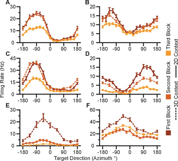
Units removed from analysis due to signal loss.

(A–E) Five units from Monkey A. (F) One unit from Monkey C. Tuning curves from the first, second, and third block of trials are shown as the curves from dark to light orange. Firing rates are drawn as the mean $\pm$ SE across the trials in the block. Blocks from the 3D context are drawn as dashed lines and those from the 2D context are drawn as solid lines. Data to recreate these plots are available in Figure 2—figure supplement 1—source data 1.

https://doi.org/10.7554/eLife.21409.007

Figure 2—figure supplement 1—source data 1 Tuning curves of neurons removed from analysis dataset.: https://doi.org/10.7554/eLife.21409.008
Download elife-21409-fig2-figsupp1-data1-v1.zip

Figure 2—figure supplement 2

Download asset Open asset

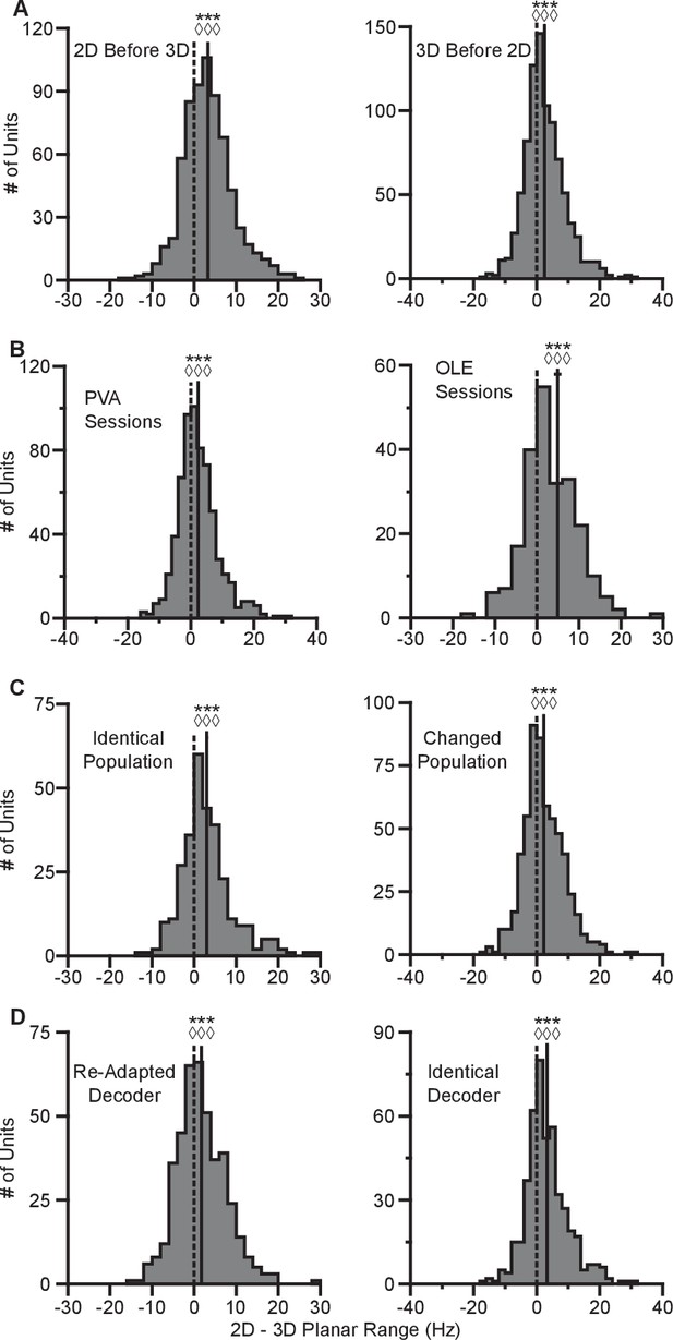
Invariance of tuning range changes.

(A) Histograms comparing the tuning ranges from both monkeys for the set of identical targets in the 2D and 3D contexts when blocks of 2D trials preceded blocks of 3D trials (left) and when blocks of 3D trials preceded blocks of 2D trials (right). $W_{l}$ = 178635, *** $P < ≪ 10^{- 38}$ , $S_{l}$ = 477, $◊ ◊ ◊ P < 10^{- 26}$ , $n_{l}$ = 671, $W_{r}$ = 273191, *** $P < 10^{- 25}$ , $S_{r}$ = 564, $◊ ◊ ◊ P < 10^{- 16}$ , $n_{r}$ = 880. $W$ , Wilcoxon signed-rank tests, $S$ , sign tests, $n$ , number of analyzed units. (B) Histograms comparing the tuning ranges for the set of identical targets in the 2D and 3D contexts for all recording sessions from both monkeys that used the PVA decoder (left) and those that used the OLE decoder (right). $W_{P V A}$ = 144603, *** $P < 10^{- 15}$ , $S_{P V A}$ = 404, $◊ ◊ ◊ P < 10^{- 9}$ , $n_{P V A}$ = 649, $W_{O L E}$ = 20273, *** $P < 10^{- 10}$ , $S_{O L E}$ = 160, $◊ ◊ ◊ P < 10^{- 8}$ , $n_{O L E}$ = 231. (C) Histograms comparing the tuning ranges from both monkeys for the set of identical targets in the 2D and 3D contexts for the subset of recording sessions where the population used for BCI control was identical between the two contexts (left) and those where the population changed (right). $W_{l}$ = 34298, *** $P < 10^{- 14}$ , $S_{l}$ = 212, $◊ ◊ ◊ P < 10^{- 11}$ , $n_{l}$ = 300, $W_{r}$ = 114164, *** $P < 10^{- 12}$ , $S_{r}$ = 352, $◊ ◊ ◊ P < 10^{- 6}$ , $n_{r}$ = 580. (D) Histograms comparing the tuning ranges for both monkeys for the set of identical targets in the 2D and 3D contexts for the subset of recording sessions where the decoder was re-adapted between the 3D and 2D contexts (left) and those were the decoder was identical with the $z$ -dimension zeroed out in the 2D context (right). $W_{l}$ = 58688, *** $P < 10^{- 6}$ , $S_{l}$ = 251, $◊ ◊ ◊ P < 10^{- 3}$ , $n_{l}$ = 425, $W_{r}$ = 78290, *** $P < 10^{- 20}$ , $S_{r} = 313$ , $◊ ◊ ◊ P < 10^{- 14}$ , $n_{r}$ = 455. For all panels: solid vertical lines, means of distributions; solid horizontal lines, mean $\pm$ SE; dashed vertical lines, point of equality between the two tuning ranges. Data to recreate these plots are available in Figure 2—figure supplement 2—source data 1.

https://doi.org/10.7554/eLife.21409.009

Figure 2—figure supplement 2—source data 1 Context order, decoder type, changed population, and re-adapted decoder tuning range dataset.: https://doi.org/10.7554/eLife.21409.010
Download elife-21409-fig2-figsupp2-data1-v1.zip

Figure 2—figure supplement 3

Download asset Open asset

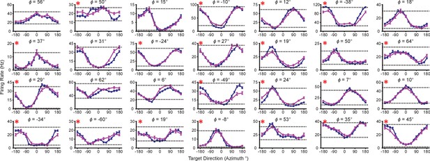
Tuning range changes for Monkey A for one recording session.

The plots show the tuning curves for the targets lying on the xy-plane in the 2D (dark blue) and 3D (pink) contexts. The firing rates are shown as the mean $\pm$ SE ( $n_{2D} = 24; n_{3 D} = 10$ ). The minimum and maximum average firing rates amongst the set of all 26 targets from the 3D context are drawn as the dotted horizontal lines. The titles above each plot show the elevation angle, $ϕ$ , that the unit’s preferred direction vector estimated from the 3D data makes with the xy-plane. Units that showed a greater tuning range amongst the set of identical targets in the 2D context than the 3D context are marked with a red asterisk at the top-left corner of the plot. Data to recreate these plots are available in Figure 2—figure supplement 3—source data 1.

https://doi.org/10.7554/eLife.21409.011

Figure 2—figure supplement 3—source data 1 Single session tuning curves dataset.: https://doi.org/10.7554/eLife.21409.012
Download elife-21409-fig2-figsupp3-data1-v1.zip

Figure 2—figure supplement 4

Download asset Open asset

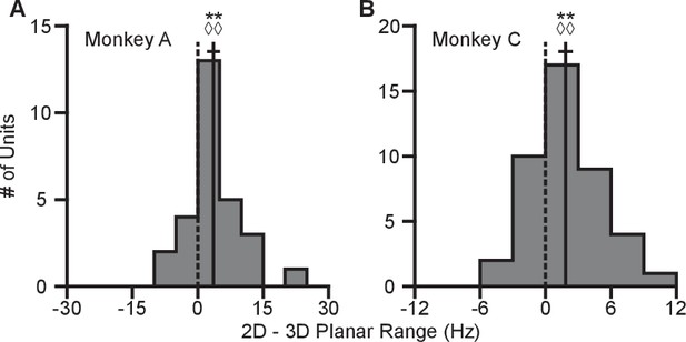
Difference in tuning ranges in single sessions.

(A,B) The plots show the histograms for the difference tuning ranges for the set of eight identical targets between the 2D and 3D contexts for Monkey A (panel A) and Monkey C (panel B) for the single recording session corresponding to the data shown in Figure 2—figure supplement 3 and a similar single recording session from Monkey C. For both panels: solid vertical lines, means of distributions; solid horizontal lines, mean $\pm$ SE; dashed vertical lines, point of equality between the two tuning ranges. $W_{A}$ = 333, ** $P = 0.0031$ , $S_{A}$ = 22, $◊ ◊ P = 0.0037$ , $n_{A}$ = 28, $W_{C}$ = 731, ** $P = 0.0018$ , $S_{C}$ = 31, $◊ ◊ P$ = 0.0054, $n_{C}$ = 43. $W$ , Wilcoxon signed-rank tests, $S$ , sign tests, $n$ , number of analyzed units. Data to recreate these plots are available in Figure 2—figure supplement 4—source data 1.

https://doi.org/10.7554/eLife.21409.013

Figure 2—figure supplement 4—source data 1 Single session tuning range dataset.: https://doi.org/10.7554/eLife.21409.014
Download elife-21409-fig2-figsupp4-data1-v1.zip

Figure 2—figure supplement 5

Download asset Open asset

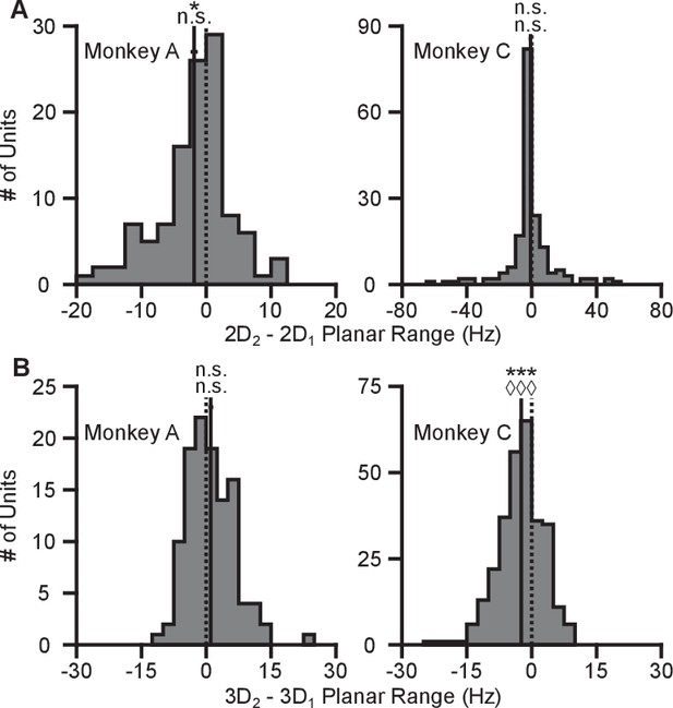
Minimal changes with repeated contexts.

(A) The plots show the histograms of the tuning range difference between repeats of the 2D context for Monkey A (left) and Monkey C (right). (B) The plots show the histograms of the tuning range difference between repeats of the 3D context for Monkey A (left) and Monkey C (right). In all plots, the difference is calculated where positive values represent increases in tuning range for the repeated context relative to the initial set of trials. For Monkey A, there is some significant difference in tuning ranges between repeats of the 2D context (2D context: * $P = 0.0047$ , $W = 2233$ , n.s. $P = 0.0904$ , $S = 47$ , $n = 113$ units; 3D context: n.s. $P = 0.1189$ , $W = 3829$ , n.s. $P = 0.6396$ , $S = 60$ , $n = 114$ units). For Monkey C, there is a significant difference in tuning ranges between repeats of the 3D context (2D context: n.s. $P = 0.2525$ , $W = 3946$ , n.s. $P = 0.0829$ , $S = 56$ , $n = 176$ units; *** $P < 10^{- 12}$ , $W = 10952$ , $◊ ◊ ◊ P < 10^{- 10}$ , $S = 88$ , $n = 291$ units). Notably, for all cases where there is a significant difference between repeat of the same context, the means lie to the left of zero. For all panels: solid vertical lines, means of distributions; solid horizontal lines, mean $\pm$ SE; dashed vertical lines, point of equality between the two tuning ranges. Data to recreate these plots are available in Figure 2—figure supplement 5—source data 1.

https://doi.org/10.7554/eLife.21409.015

Figure 2—figure supplement 5—source data 1 Repeat context tuning range dataset.: https://doi.org/10.7554/eLife.21409.016
Download elife-21409-fig2-figsupp5-data1-v1.zip

Figure 3

Download asset Open asset

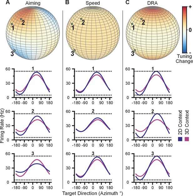
Hypotheses for tuning changes.

(A) Illustration of the re-aiming strategy hypothesis. (B) Illustration of the speed hypothesis. (C) Illustration of the dynamic range adaptation hypothesis. For each hypothesis, the first row shows heat maps of the relative change in tuning range as a function of preferred direction. For illustrative purposes, the heat map in (panel A) is shown as $\frac{2 D R a n g e - 3 D P l a n a r R a n g e}{3 D R a n g e}$ and scaled in the range $[- 0.25, 0.25]$ . The other heat maps are shown as $1 - \frac{3 D P l a n a r R a n g e}{2 D R a n g e}$ and scaled in the range $[- 1, 1]$ . The bottom three rows show example changes in tuning functions for three units with preferred directions drawn as the light green points on the heat maps.

https://doi.org/10.7554/eLife.21409.017

Figure 4 with 1 supplement

Download asset Open asset

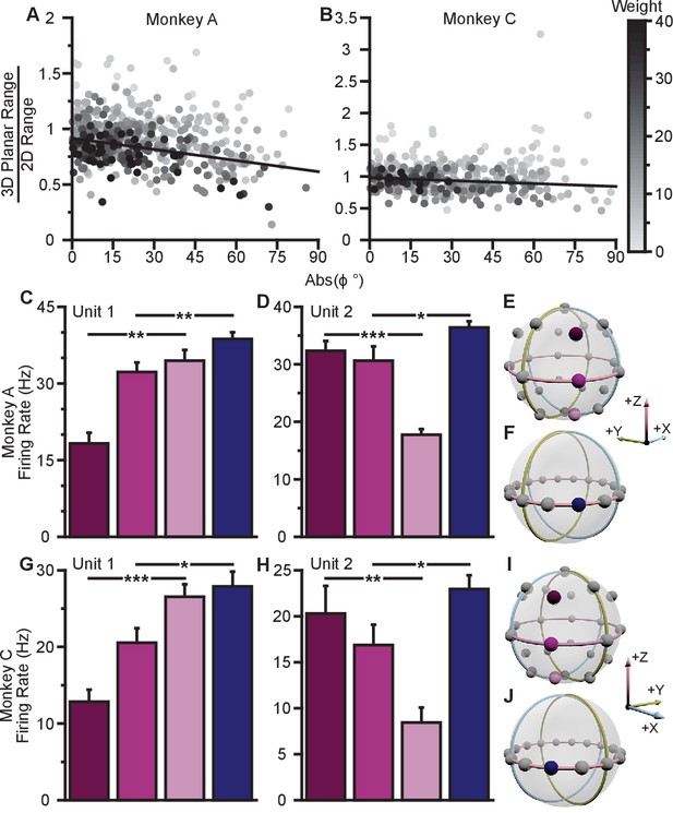
Evidence for dynamic range adaptation.

(A) Dose-response effects in the tuning changes for Monkey A. (B) Dose-response effects in the tuning changes for Monkey C. The ratio of 3D planar to 2D dynamic ranges are plotted against the absolute value of the elevation angle ( $ϕ$ ) of the PD vectors. The weighted linear fits for the data points are shown in black. The fits have negative slopes. $b_{A} = - 0.0033$ , $F_{A} = 53.9$ , $P < 10^{- 12}$ , $n_{A} = 471$ , $b_{C} = - 0.0015$ , $F_{C} = 10.6$ , $P = 0.00125$ , $n_{C} = 409. b$ , slope, $F$ , $F$ -test versus constant model, $n$ , number of analyzed units. The darkness of the points corresponds to the weights used for the linear fits with the legend shown to the right. To provide contrast, the upper threshold of colormap for the weights was set at 40. The tuning curves for the two points that lie significantly off the trend line in (B) are shown in Figure 4—figure supplement 1B. (C,D) Firing rates from Monkey A for the first two units from Figure 2A. Both units have an azimuthal PD near $- 135^{\circ}$ . The first three bars show the firing rates in the 3D context for the target that lay at $- 135^{\circ}$ on the xy-plane (pink) and the two targets immediately above (dark pink), and below (light pink) that target (E). The firing rate in the 2D context to the target at $- 135^{\circ}$ is shown in the fourth bar (F). Unit 1 had a preferred direction below the xy-plane ( $U_{1; Z} = 61$ , ** $P = 0.001$ ). Unit 2 had a preferred direction above the xy-plane ( $U_{2; Z} = 154$ , *** $P < 10^{- 3}$ ). Despite this difference, both units showed an increased firing rate to the planar target in the 2D context compared to the 3D context ( $U_{1; 2 D, 3 D} = 114$ , ** $P = 0.0098$ , $U_{2; 2 D, 3 D} = 126$ , * $P = 0.0299$ ). (G,H) Similar set of firing rates from Monkey C for the first two units from Figure 2B. The corresponding targets are shown in (I and J). Both units had an azimuthal PD near $- 45^{\circ}$ . Unit 1 had a preferred direction below the xy-plane $U_{1; Z} = 69$ , *** $P < 10^{- 3}$ ). Unit 2 had a preferred direction above the xy-plane ( $U_{2; Z} = 164$ , ** $P = 0.0028$ ). Despite this difference, both units showed an increased firing rate to the planar target in the 2D context compared to the 3D context ( $U_{1; 2 D, 3 D} = 89$ , * $P = 0.0165$ , $U_{2; 2 D, 3 D} = 95$ , * $P = 0.0374$ ). The firing rates are plotted as the mean $\pm$ SE ( $U$ , Mann-Whitney $U$ tests, $n_{2 D}$ and $n_{3 D}$ trials are the same from Figure 2A,B). Data to recreate these plots are available in Figure 4—source data 1.

https://doi.org/10.7554/eLife.21409.018

Figure 4—source data 1 Tuning range change versus elevation angles and paired neuron changes dataset.: https://doi.org/10.7554/eLife.21409.019
Download elife-21409-fig4-data1-v1.zip

Figure 4—figure supplement 1

Download asset Open asset

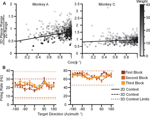
Dose-response effects in firing rate changes.

(A) Dose-response effects in the tuning changes are shown for Monkey A (left) and Monkey C (right). The ratio of 3D planar to 2D dynamic ranges are plotted against the cosine of the elevation angle ( $ϕ$ ) of the PD vectors. The weighted linear fits for the data points are shown in black. The fits have positive slopes. $b_{A} = 0.397$ , $F_{A} = 63.6$ , $P < 10^{- 13}$ , $n_{A} = 471$ , $b_{C} = 0.152$ , $F_{C} = 8.92$ , $P = 0.00299$ , $n_{C} = 409. b$ , slope, $F$ , $F$ -test versus constant model, $n$ , number of analyzed units. The darkness of the points corresponds to the weights used for the linear fits with the legend shown to the right. To provide contrast, the upper threshold of colormap for the weights was set at 40. (B) The tuning curves for the two points that lie significantly off the trend line for Monkey C. The plots show the tuning curves for the targets lying on the xy-plane in the 2D (solid line) and 3D (dashed line) contexts. The firing rates are shown as the mean $\pm$ SE. The minimum and maximum average firing rates amongst the set of all 26 targets from the 3D context are drawn as the dotted horizontal lines. The tuning curves and the minimum and maximum lines are colored (dark to light orange) according to the block order of the data (first to third block). The tuning curves show a noisy response to targets in the xy-plane with decreased estimated ranges in the 2D context. Data to recreate these plots are available in Figure 4—figure supplement 1—source data 1.

https://doi.org/10.7554/eLife.21409.020

Figure 4—figure supplement 1—source data 1 Tuning range change versus elevation angles and outlier neural tuning curves dataset.: https://doi.org/10.7554/eLife.21409.021
Download elife-21409-fig4-figsupp1-data1-v1.zip

Figure 5

Download asset Open asset

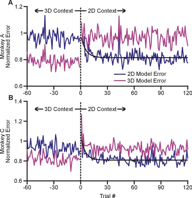
Time course of adaptation.

The two panels show the time courses of adaptation for Monkey A (A) and Monkey B (B). The ordinate axes in the plots show the standardized error between the firing rates in the population and the expected response from tuning fits. Each plot shows two different errors: the error based on tuning models from the 2D context (dark blue) and from the 3D context (pink). These standardized errors are averaged across multiple recording sessions for Monkey A (18) and Monkey C (11). The abscissa in the plots show the trial number before and after the change from the 3D context to the 2D context. The data points to the right of zero represent the standardized error for the first 120 trials in the 2D context. The data points to the left of zero represent the last 60 planar target trials of the the 3D context. The dashed black vertical line at zero represents the system down-time while the context was switched. We also plotted exponential fits (black) to the 2D tuning model error for the first 120 trials of the 2D context. The data were fit to the equation: $y = a + b \exp c x$ . For Monkey A, the fit parameters (with 95% confidence bounds) were: a = 0.815(0.807, 0.8233); b = 0.176(0.087, 0.264); c = −0.189(−0.317, −0.060); r² = 0.229. For Monkey C, the fit parameters were: a = 0.809(0.800,0.818); b = 0.250(0.150, 0.348); c = −0.202(−0.309, −0.095); r² = 0.328. Data to recreate these plots is available in Figure 5—source data 1.

https://doi.org/10.7554/eLife.21409.022

Figure 5—source data 1 Trial-by-trial tuning model error dataset.: https://doi.org/10.7554/eLife.21409.023
Download elife-21409-fig5-data1-v1.zip

Figure 6

Download asset Open asset

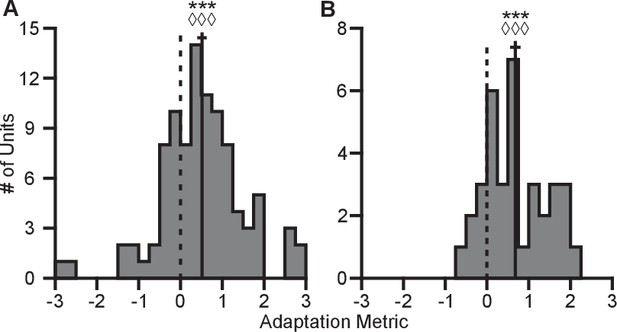
Completeness of adaptation.

The two panels show histograms of the completeness metric for Monkey A (A) and Monkey C (B). For both panels: solid vertical lines, means of distributions; solid horizontal lines, mean $\pm$ SE; dashed vertical lines, zero point representing no dynamic range adaptation. For both monkeys, histograms were distributed significantly away from the zero point (Monkey A: *** $P < 10^{- 5}$ , Wilcoxon signed-rank test, $W = 3580$ , $◊ ◊ ◊ P < 10^{- 3}$ , sign test, $S = 68$ , $n = 95$ units; Monkey C: *** $P < 10^{- 4}$ , $W = 570$ , $◊ ◊ ◊ P < 10^{- 3}$ , $S = 29$ , $n = 35$ units). The means ( $\pm$ SE) of the metrics were 0.5157 ( $\pm$ 0.1121) for Monkey A and 0.6793 ( $\pm$ 0.1233) for Monkey C. Data to recreate these plots is available in Figure 6—source data 1.

https://doi.org/10.7554/eLife.21409.024

Figure 6—source data 1 Adaptation metric dataset.: https://doi.org/10.7554/eLife.21409.025
Download elife-21409-fig6-data1-v1.zip

Figure 7

Download asset Open asset

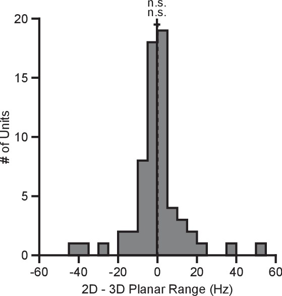
Tuning range in hand-control task.

The plot shows the histogram of the tuning range difference between the 2D and 3D contexts for the planar targets in the hand-control task. For the plot: solid vertical line, mean of distribution; solid horizontal line, mean $\pm$ SE; dashed vertical line, point of equality between the two tuning ranges. For Monkey N, the tuning ranges were not significantly different between the 2D and 3D contexts (n.s. $P = 0.6349$ , Wilcoxon signed-rank test, $W = 969$ , n.s. $P = 0.9007$ , $S = 31$ , $n = 64$ units). Data to recreate these plots are available in Figure 7—source data 1.

https://doi.org/10.7554/eLife.21409.026

Figure 7—source data 1 Hand-control task tuning range dataset.: https://doi.org/10.7554/eLife.21409.027
Download elife-21409-fig7-data1-v1.zip

Download links

A two-part list of links to download the article, or parts of the article, in various formats.

Downloads (link to download the article as PDF)

Open citations (links to open the citations from this article in various online reference manager services)

Mendeley

Cite this article (links to download the citations from this article in formats compatible with various reference manager tools)

Robert G Rasmussen
Andrew Schwartz
Steven M Chase

(2017)

Dynamic range adaptation in primary motor cortical populations

eLife 6:e21409.

https://doi.org/10.7554/eLife.21409

Sign up for email alerts

Privacy notice