Mapping the function of neuronal ion channels in model and experiment
- University of Oxford, United Kingdom
- École Polytechnique Fédérale de Lausanne, Switzerland
- Ecole Polytechnique Federale de Lausanne, Switzerland
Figures
Figure 1
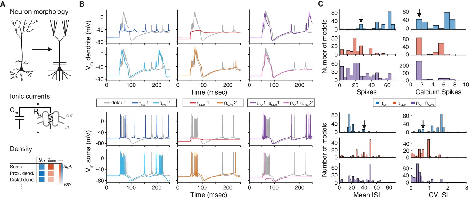
The choice of ion channel model influences the behavior of a simulated neuron.
(A) Biophysical neuron models are composed of a detailed multicompartmental morphology, several active ion channel conductances, and a density of each conductance that depends on the specific compartment. (B) Simulation of a detailed layer 2/3 pyramidal neuron model, adapted from Traub et al. (2003) (see Materials and methods for details). The neuron model was stimulated with a 1.5 nA current step beginning at 50 ms, while recording the membrane potential in the apical dendrite (top) and soma (bottom). Simulations were first run using the original conductances from Traub et al. (‘default’, gray). Left: the default A-type potassium model () was replaced with two other A-type models (1: dark blue, Hay et al. [2011], ModelDB ID no. 139653; 2: light blue, Traub et al. [2005], ModelDB ID no. 45539). Middle: the default delayed rectifier potassium model () was replaced with two other delayed rectifier models (1: red, Zhou and Hablitz [1996], ModelDB ID no. 3660; : orange, Durstewitz et al. [2000], ModelDB ID no. 82849). Right: both A-type and delayed rectifier models were replaced with other models (1 + 1, purple; 1 + 2, magenta). (C) Model from B was simulated for 1000 ms with a 1.5 nA current step. Firstly, the default A-type current model was replaced with each of the 243 A-type-labeled model on ModelDB (blue). Secondly, the default delayed rectified current was replaced with each of the 188 delayed rectifier models on ModelDB (red). Finally, the default A-type and delayed rectifier currents were replaced with a random sample of approximately 1% of all possible combinations of A-type and delayed rectifier models on ModelDB (purple). Summary measures are shown for total number of spikes, total number of calcium spikes, mean inter-spike interval (ISI) and coefficient of variation (CV) of ISI during the 1000 ms period. Black arrows represent the simulation results for the default model.
Figure 2
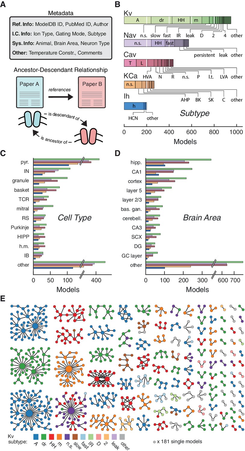
Ion channel models can be categorized by metadata and ancestor-descendant relationships.
(A) Metadata were manually extracted from ModelDB and associated journal articles (top). Ancestor-descendant relationship (bottom) was established between different models (see main text for description). (B) Models were divided into five classes based on ion type: voltage-dependent potassium (Kv), voltage-dependent sodium (Nav), voltage-dependent calcium (Cav), calcium-dependent potassium (KCa), and hyperpolarization-activated cation (Ih). Each class is divided into subtypes, ordered from left to right according to group size. Uncommon subtypes are grouped together (other). (C, D) Histogram of cell types and brain areas for each ion type, ordered from top to bottom by the number of models. Colors as in B. (E) Pedigree graph displaying families of the Kv class, sorted by family size. Each node represents one model, colored by subtype, and edges represent ancestral relations between models (panel A, bottom). Note that unconnected models (181 total) are not shown. A: A-type, dr: delayed rectifier, HH: Hodgkin-Huxley, m: m-type, n.s.: not specified, IR: inward rectifier, HVA: high-voltage activating, N: N-type, R: R-type, P: P-type, l.t.: low threshold, LVA: low-voltage activating, AHP: after-hyperpolarization, BK: big conductance, SK: small conductance, HCN: Hyperpolarization-activated cyclic nucleotide-gated, pyr.: pyramidal, IN: interneuron, TCR: thalamocortical relay, RS: regular spiking, HIPP: hilar perforant-path associated, h.m.: hilar mossy, IB: intrinsic bursting, hipp: hippocampus, bas. gan.: basal ganglia, cerebell.: cerebellum, SCX: somatosensory cortex, DG: dentate gyrus, GC: granule cell.
-
Figure 2—source data 1
Table of subtypes for each ion type class.
Subtypes of each of the five classes currently available in the resource (Kv, Nav, Cav, KCa, Ih), sorted by the frequency of their occurrence.
- https://doi.org/10.7554/eLife.22152.004
Figure 3 with 4 supplements
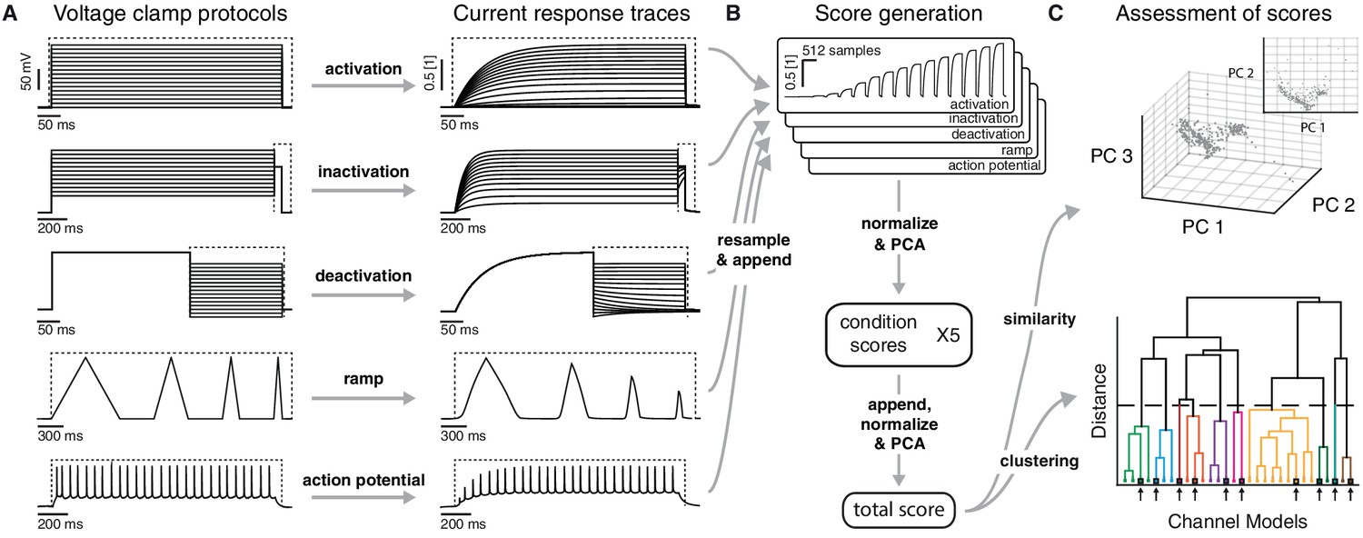
Voltage-clamp protocols for the quantitative analysis of ion channel models.
(A) Left: five voltage clamp protocols were used to characterize ion channel responses recorded in single compartment somata simulated in NEURON (see Figure 3—figure supplement 1 and Tables 1 and 2 for full description). Multiple lines indicate a series of increasing voltage steps with the same time sequence. Right: current response traces are shown for an example model. Dashed regions indicate response times used for data analysis. (B) Current responses were subsampled and appended, then dimensionality-reduced by principal component analysis (PCA) to form a condition score vector for each protocol. These score vectors were further normalized and dimensionality-reduced to form a total score vector. (C) The first three principal components of the score vector are shown for Kv ion channel models (top). Scores were clustered using an agglomerative hierarchical clustering technique (bottom). Distinct clusters (noted by colors) form when a cutoff (dashed line) is introduced in the distance between hierarchical groupings, chosen based on several cluster indexes (see Figure 3—figure supplements 2 and 3). Cluster representative models (bold squares with arrows) are selected as reference models for each cluster (see Materials and methods).
-
Figure 3—source data 1
Table of omitted files.
List of omitted files for each of the five ion type classes, with a brief description of the reason for omission.
- https://doi.org/10.7554/eLife.22152.006
Figure 3—figure supplement 1
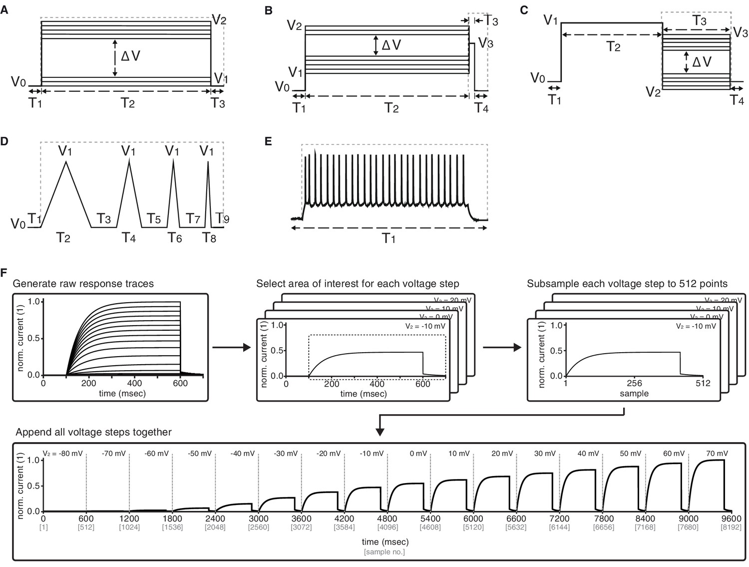
Graphical description of the five voltage-clamp protocols used for ion channel model analysis.
Activation (A), inactivation (B), deactivation (C), ramp (D), action potential (E). See Table 2 for values of variables used in simulations. Dashed lines represent the approximate regions used for analysis. (F) Preprocessing stage of analysis – example shown for Kv activation protocol. Raw current response traces are cut to include only the region inside the dashed lines (as in panels A-E) for each of the (sixteen, for activation) voltage steps of the protocol. Then, each of the resulting traces is separately subsampled to obtain 512 data points. Finally, the subsampled traces are appended to form a final vector of size . Other protocols for Kv and the other four classes are processed similarly, with the following two comments: (1) ramp and action potential protocols do not feature multiple voltage steps, and so only contain 512 datapoints total; (2) KCa current traces are run at seven different calcium concentrations, which are processed separately for each concentration as shown here, and then appended together – e.g., KCa activation will contain data points.
Figure 3—figure supplement 2
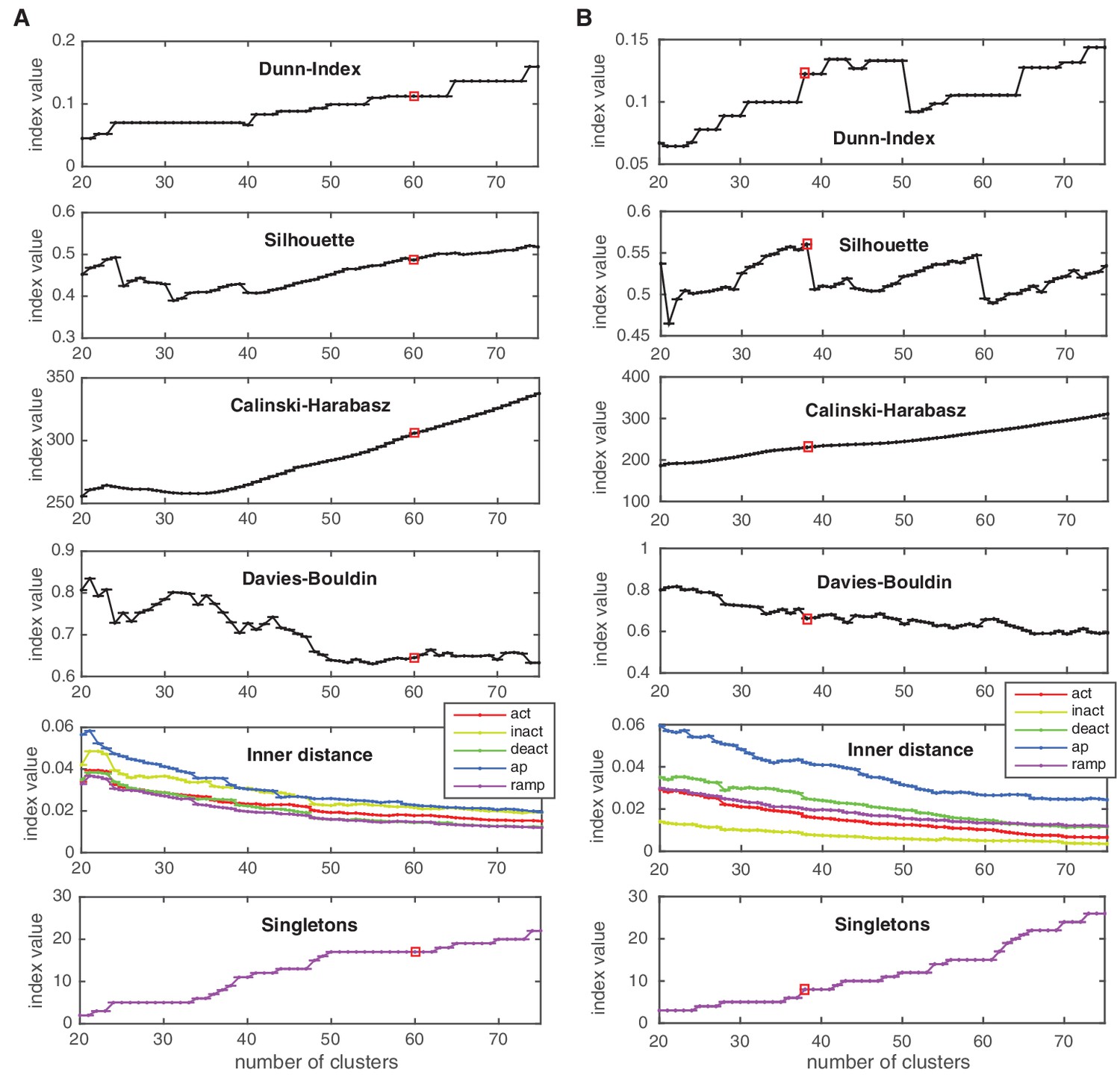
Cluster indexes for Kv and Nav classes.
See Materials and methods for description. ‘Singletons’ refers to the number of single-element clusters. (A) Cluster indexes of the Kv class. The cluster number 60 was chosen since Dunn and Silhouette indexes display a large value, Calinski-Harabasz displays a ‘knee’ (decrease in steepness) while the Davies-Bouldin is close to a local minimum. Candidate numbers 55 (Davies-Bouldin minimum) and 59 (local maximum of Silhouette, decrease in the inner distance of all conditions) were disregarded due to the lower Silhouette index, and since a splitting of a major A-type cluster into two distinct clusters was observed at 60. (B) Cluster indexes of the Nav class. The cluster number 38 was chosen since Calinski-Harabasz displays a ‘knee’ (decrease in steepness), the Dunn index displays a sharp increase, the Silhouette index a sharp decrease for higher numbers, and the inner distance displays a slight decrease in all conditions. The chosen cluster number is indicated by a red box.
Figure 3—figure supplement 3
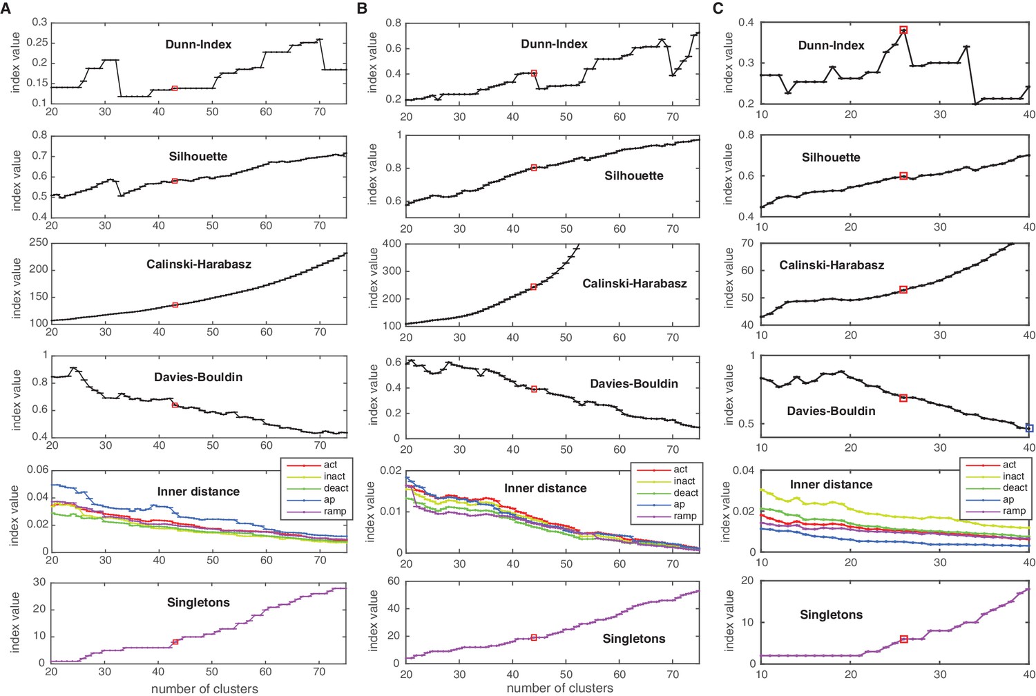
Cluster indexes for Cav, KCa and Ih classes.
Cluster indexes, see Materials and methods for description. ‘Singletons’ refers to the number of single-element clusters. (A) Cluster indexes of the Cav class. The candidate cluster number 30 (peak of Dunn-index and Silhouette, local minimum of Davies-Bouldin) was disregarded since clusters were too heterogeneous (large inner distance). The next candidate cluster number 43 was chosen instead (Dunn and Silhouette display a local increase), Calinski-Harabasz displays a slight ‘knee’ (decrease in steepness) and Davies-Bouldin displays a sharp drop. Also, a sharp decrease in ‘action potential’ (ap) inner distance is visible at cluster number 43. (B) Cluster indexes of the KCa class. The cluster number 44 was chosen since Calinski-Harabasz displays a slight ‘knee’ (decrease in steepness), the Dunn index displays an increase before a sharp drop while the Silhouette increases over the candidate number of 41. Also, Davies-Bouldin, stops decreasing and the inner distance displays a decrease in all conditions. (C) Cluster indexes of the Ih class. The cluster number 26 was chosen since the Dunn index displays a clear local maximum, as does the Silhouette, while Davies-Bouldin stops decreasing. The candidate number 27 (Calinski-Harabasz displays a clear ‘knee’) was disregarded, since the other indexes all show unfavorable changes. The chosen cluster number is indicated by a red box.
Figure 3—figure supplement 4

Comparison of intra- and inter-subtype variability with intra- and inter-cluster variability.
(A) Median pairwise distance between all channels of a given subtype, calculated either with the final score (‘total’), or only each of the intermediate condition scores (here abbreviated, cf. Figure 3). The distance is given with respect to subtype given in each column, that is, the first column displays the distance of channels of all other subtypes to the A subtype. Black circles display the median pairwise distance between those channels of a given subtype that are in the same clusters. All distances are normalized by the pairwise median distance averaged over all displayed subtypes. This shows that, e.g., A differs from other subtypes in all but the action potential protocol, while for example the m-type label differs from all other subtypes mostly in the action potential protocol. The clustering reduces the median variability to much lower levels than just the subtype partition, as visible in the black dots of each plot. Numbers in parentheses show the number of channels in the given subtype. (B) Same as in A, however pairwise distances are calculated for channels in the given clusters. The distance is given with respect to the cluster in each column, that is, the first column displays the distance of channels in all clusters to channels in cluster 33. The first two clusters consist mostly of A-type channels (33: 80%,1: 91%), the middle two clusters comprise primarily of HH/dr channels (20: 36% HH/55% dr, 10: 39% HH/55% dr), and the right two clusters consist mostly of m-type channels (47: 73%,48: 73%). Numbers in parentheses correspond to the number of unique channels in the given cluster. C Mean current response traces of the clusters in panel B. The insets marked by a, b, c are zooms of parts of the response traces, enlarged to clarify regions of distinct current responses.
Figure 4 with 2 supplements
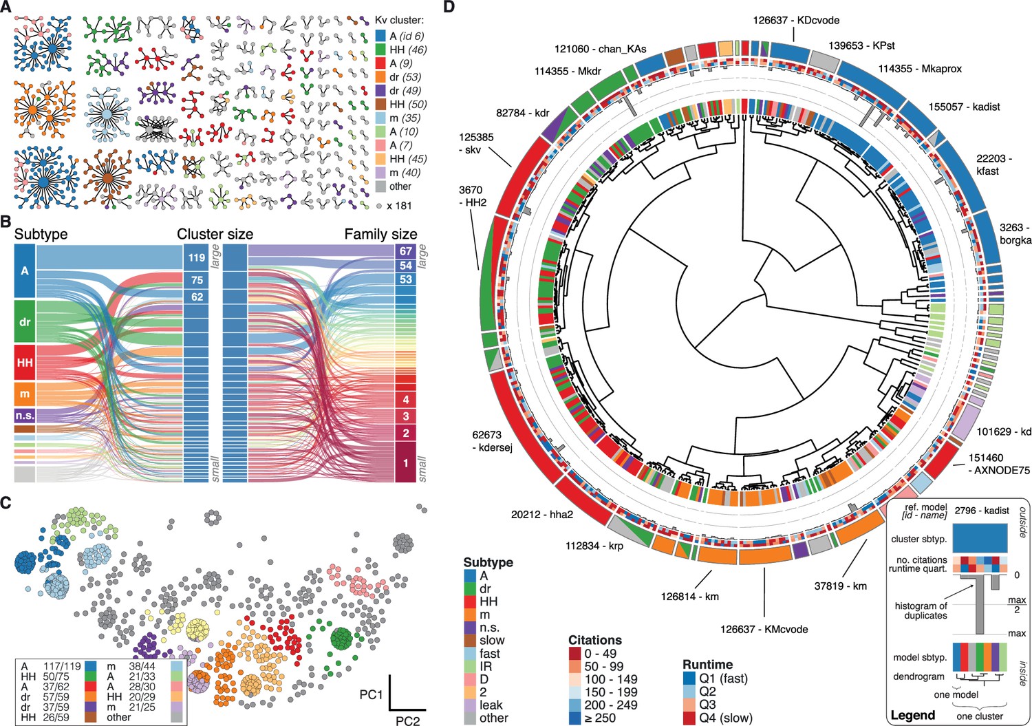
Quantitative analysis of Kv ion channel models: functional map and clusters of common behavior.
(A) Pedigree graph of the Kv class (cf. Figure 2E), colored by membership in the 11 largest clusters in the class (named by most prevalent subtype, bottom). Membership to other clusters is indicated by gray color. Cluster ID is given in parentheses for easy comparison with website. (B) ‘Sankey’ diagram for the Kv ion type class, showing the relation between subtype, cluster identification and family identification, each ordered from top to bottom by increasing group size. The 11 most common subtypes are shown in color, with all others grouped together in gray. Small families (size 1 to 6 members) are grouped together. (C) Plot of Kv models in the first two principal components of score space. Colors indicate membership in one of the 11 largest clusters in the class, with membership to other clusters colored in gray. Clusters are named by their most common subtype, with the proportion of that subtype specified in the legend. Points lying very close to each other have been distributed around the original coordinate for visualization. (D) ‘Circos’ diagram of the Kv ion type class. All unique ion channel models are displayed on a ring, organized by cluster identification. From outside to inside, each segment specifies: cluster reference model (only displayed for large clusters), cluster subtype(s) (all subtype labels that contribute at least ), number of citations, runtime, number of duplicates, model subtype, as well as a dendrogram of cluster connections (black) and family relations (gray). A: A-type, dr: delayed rectifier, HH: Hodgkin-Huxley, m: m-type, n.s.: not specified, IR: inward rectifier. See Figure 4—figure supplements 1 and 2 for other ion type classes.
Figure 4—figure supplement 1
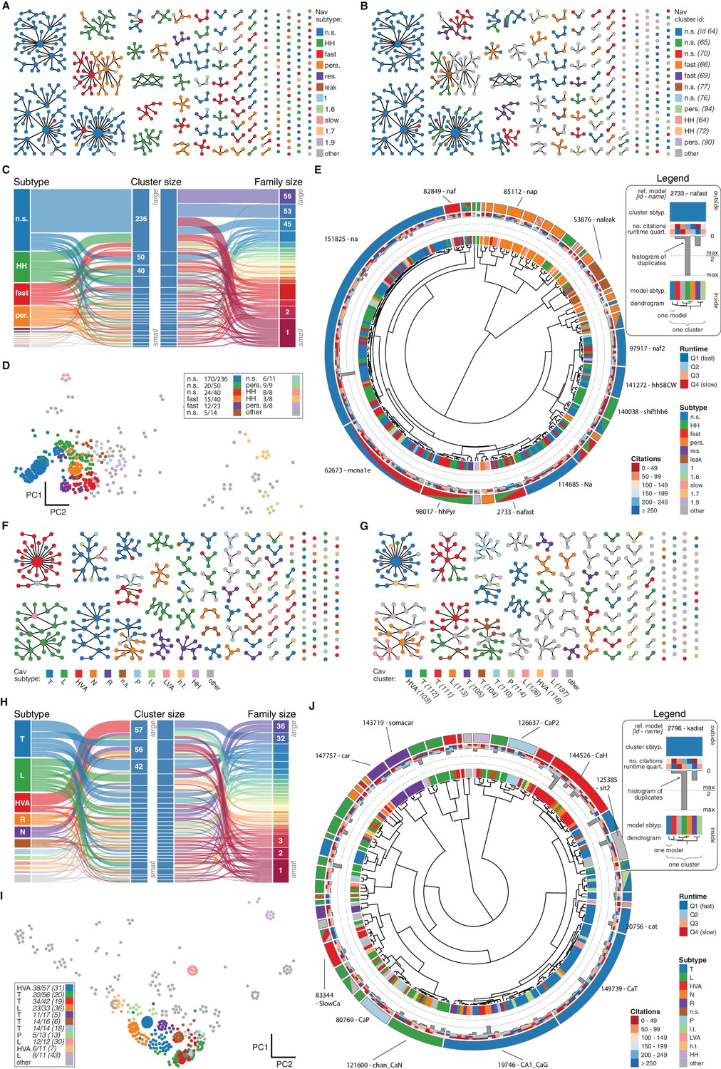
Nav and Cav class genealogy and clustering.
(A) Families of the Nav class, ordered from left to right by family size. Each dot represents an ion channel model and edges represent family relationships. Colors indicate the 11 most prevalent subtypes in the class, with other subtypes colored in gray. (B) Families of the Nav class, as in panel A. Colors indicate membership in one of the 11 largest clusters in the class (named by most prevalent subtype, right hand side), with membership to other clusters colored in gray. Cluster ID is given for easy comparison with website. (C) ‘Sankey’ diagram for the Nav ion type class, showing the relation between subtype, cluster identification and family identification, each ordered from top to bottom by increasing size. The 11 most common subtypes are shown, with others being grouped together (gray). Small families (size 1 to 5 members) are grouped together. (D) Plot of Nav models in the first two principal components of score space. Colors indicate membership in one of the 11 largest clusters in the class, with membership to other clusters colored in gray. Legend indicates the most common subtype in each cluster, and the proportion of models with that subtype. Points lying very close to each other have been distributed around the original coordinate for visualization purposes. (E) ‘Circos’ diagram of the Nav ion type class. All unique ion channel models are displayed on a ring, organized by cluster identification. From outside to inside, each segment specifies: cluster reference model (only displayed for large clusters), cluster subtype, number of citations, runtime, number of duplicates, model subtype, as well as a dendrogram of cluster connections (black) and family relations (gray). n.s.: not specified, HH: Hodgkin-Huxley, per./pers.: persistent, res.: resurgent. (F–J): Cav family, similar to panels A-E. T: T-type, L: L-type, HVA: high-voltage activated, N: N-type, R: R-type, n.s.: not specified, P: P-type, l.t.: low threshold, LVA: low-voltage activated, h.t.: high threshold.
Figure 4—figure supplement 2
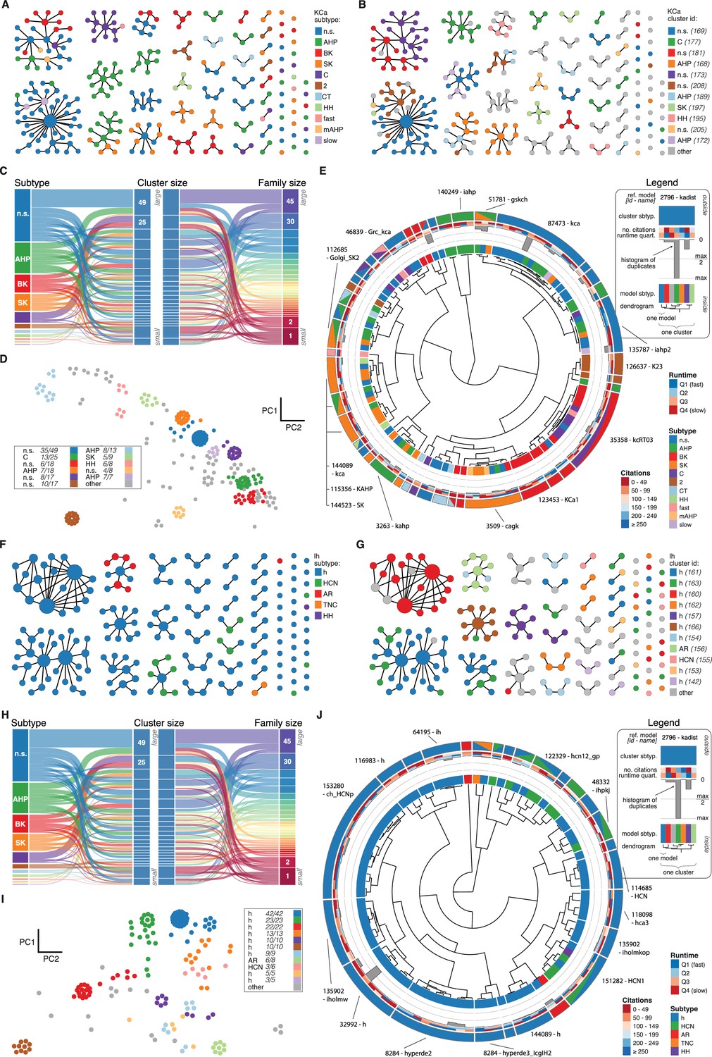
KCa and Ih class genealogy and clustering.
(A) Families of the KCa class, ordered from left to right by family size. Each dot represents an ion channel model and edges represent family relationships. Colors indicate the 11 subtypes in the class. (B) Families of the KCa class, as in panel A. Colors indicate membership in one of the 11 largest clusters in the class (named by most prevalent subtype, right hand side), with membership to other clusters colored in gray. Cluster ID is given for easy comparison with website. (C) ‘Sankey’ diagram for the KCa ion type class, showing the relation between subtype, cluster identification and family identification, each ordered from top to bottom by increasing size. Small families (size 1 to 2 members) are grouped together. (D) Plot of KCa models in the first two principal components of score space. Colors indicate membership in one of the 11 largest clusters in the class, with membership to other clusters colored in gray. Legend indicates the most common subtype in each cluster, and the proportion of models with that subtype. Points lying very close to each other have been distributed around the original coordinate for visualization purposes. (E) ‘Circos’ diagram of the KCa ion type class. All unique ion channel models are displayed on a ring, organized by cluster identification. From outside to inside, each segment specifies: cluster reference model (only displayed for large clusters), cluster subtype, number of citations, runtime, number of duplicates, model subtype, as well as a dendrogram of cluster connections (black) and family relations (gray). n.s.: not specified, AHP: after-hyperpolarization, BK: big conductance, SK: small conductance, HH: Hodgkin-Huxley, mAHP: medium AHP. (F–J): Ih family, similar to panels A-E. h: hyperpolarization-activated, HCN: hyperpolarization-activated cyclic nucleotide-gated, AR: anomalous rectifier, TNC: tonic nonspecific current.
Figure 5
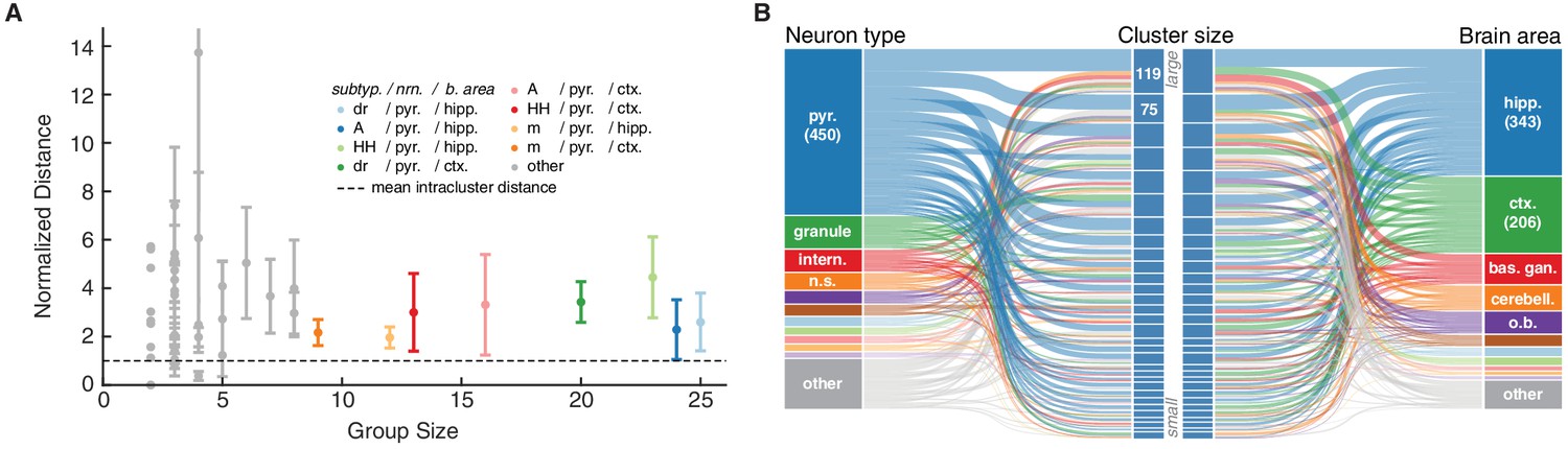
Ion channel model groups defined by common subtype, neuron type and brain area show variability in behavior.
(A) Kv models are grouped by common subtype, neuron type, and brain area. The mean pairwise distance in score space between all models within a group is plotted against group size, with errorbars corresponding to the first and third quartiles (middle 50% of distances). The largest eight groups are shown in color. Distances are normalized relative to the mean pairwise distance between models in the same cluster (dashed line; averaged across all clusters with at least one pairwise distance greater than zero, 43 of 60 clusters). Most groups have a larger mean distance than the average cluster (above the dashed line). (B) ‘Sankey’ relational diagram for metadata, neuron type, cluster identification and brain area, for the Kv ion type class. Bars are stacked histograms, that is, the height of the bars indicates the relative number of models. Left column: partition of channels by 11 most prevalent neuron types. Middle column: partition of channels into assigned clusters. Right column: partition of channels by 11 most prevalent brain areas. Links between columns are colored according to neuron type (left) and brain area (right). Numbers in the left/right column are the number of channels per label. pyr: pyramidal, intern.: interneuron, n.s.: not specified, hipp.: hippocampus, ctx: cortex, bas. gan.: basal ganglia, cerebell: cerebellum, o.b.: olfactory bulb.
Figure 6 with 1 supplement
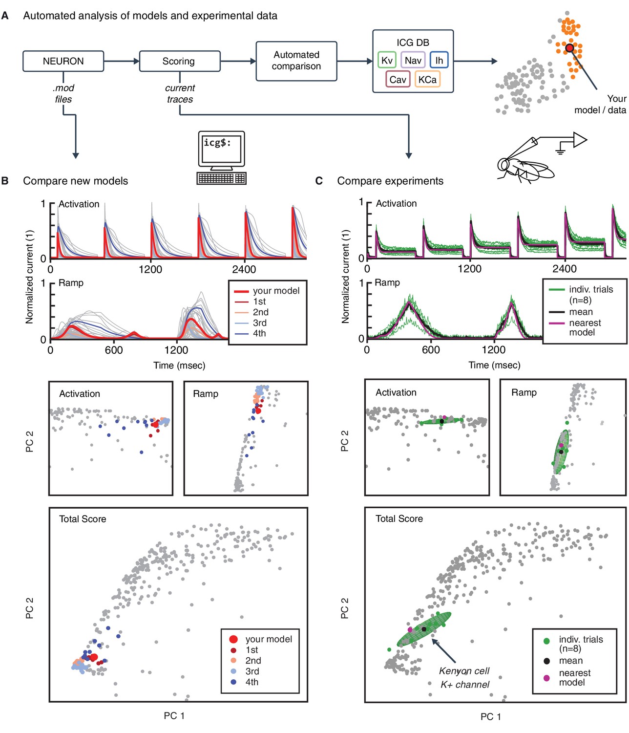
Automated analysis of new models and experimental data.
(A) Flowchart of data processing steps involved in automated comparison. Source code for model files written in NEURON can be uploaded to the website, and current responses are automatically generated. Current traces are processed to compute scores, which are compared to all models in the resource (illustrated in B). Additionally, raw current traces obtained experimentally (or from models in other languages) can be uploaded and analyzed directly (illustrated in C). (B) Example analysis and comparison of a new ion channel model (kad.mod from Hsu et al. (2015); ModelDB ID no. 184054). Top: Segments of the current response traces (red) for activation (voltage steps 10–60 mV) and ramp protocols (first half), along with the closest four clusters (other colors: mean currents, gray lines: individual currents). Bottom: first two principal components of score space for activation and ramp protocols, as well as total score. (C) Example analysis of in vivo recordings of a K+ current from Drosophila Kenyon cells (see Materials and methods for details and Figure 6—figure supplement 1 for full traces) and comparison to ICG resource. Top: mean (n = 8 recordings, black) and individual recordings (green). Bottom: mean (black dot) and individual experimental recordings (green dots) plotted in the first two principal components of score space (ellipsoid illustrates the variance across individual recordings). Comparison is made to the nearest (in score space) ion channel model in the resource (magenta; Kv4_csi, ModelDB ID no. 145672). Gray dots in B and C are scores of Kv channel models in the resource.
Figure 6—figure supplement 1
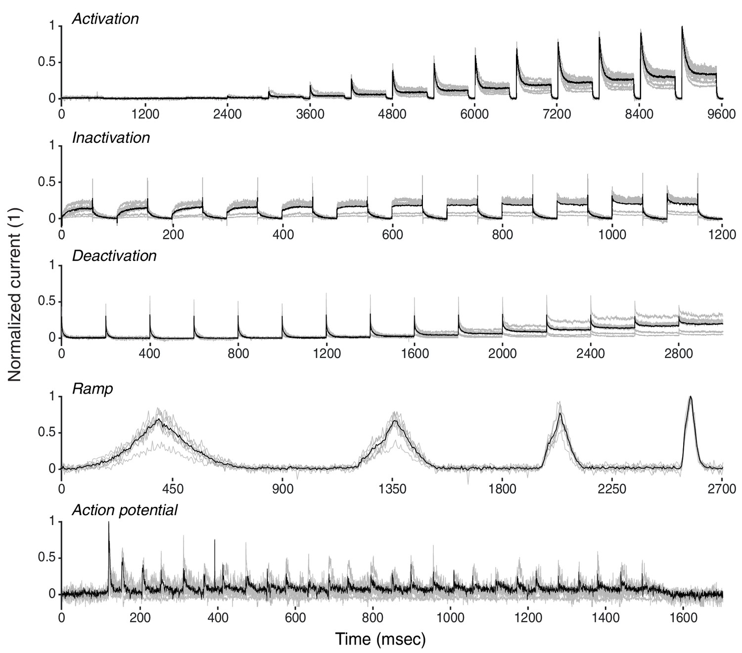
K+ current recordings from Drosophila Kenyon cells.
Recordings from eight example traces of K+ current from Drosophila Kenyon cells (gray), with average (black). See Materials and methods for a description of experiments. Response traces are arranged as detailed in Figure 3—figure supplements 1,3.
Figure 7
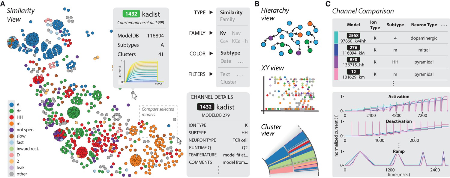
The ICGenealogy website allows for the interactive visualization of all data and analysis on the resource (ICGenealogy, 2016) (http://icg.neurotheory.ox.ac.uk).
(A) Schematic of similarity view on website. Channel models of the Kv family are displayed in the first two principal components of score space, colored by subtype (legend on left). Hovering over models brings up information tooltip (center), and clicking on a model displays Channel Details (bottom right). Selected models can be compared by click-and-drag (see instruction manual in Supplementary file 1 for more details). (B) Schematic of other three views available on the website. Hierarchy view: models are displayed in a graph with edges that represent family relations. XY view: any two selected metadata are plotted against each other. Cluster view: models are organized in a ring partitioned by clusters. (C) The channel comparison displays selected channels side-by-side with metadata (top) and current responses (bottom).
Tables
Table 1
Parameters for reversal potential and inside and outside concentrations used in simulation protocols for five ion type classes. Ionic concentrations were not used for Ih currents.
| (mV) | (mM) | (mM) | |
|---|---|---|---|
| Kv | −86.7 | 85.0 | 3.3152396 |
| Nav | 50.0 | 21.0 | 136.3753955 |
| Cav | 135.0 | 8.1929e-5 | 2.0 |
| KCa | −86.7 | 85.0 | 3.3152396 |
| Ih | −45.0 | − | − |
Table 2
Voltage-clamp protocol parameters for the five ion type classes. Times are stated in units of ms, voltages in units of mV. See Figure 3—figure supplement 1 for graphical description. Items and represent the starting and ending times, respectively, of the regions used for analysis (dashed areas in Figure 3 of the main text, as well as Figure 3—figure supplement 1).
| Act | Ion type | |||||||||||||
|---|---|---|---|---|---|---|---|---|---|---|---|---|---|---|
| Kv | −80 | −80 | 70 | 10 | 100 | 500 | 100 | 100 | 700 | |||||
| Nav | −80 | −80 | 70 | 10 | 20 | 50 | 30 | 18 | 100 | |||||
| Cav | −80 | −80 | 70 | 10 | 100 | 500 | 100 | 98 | 700 | |||||
| KCa | −80 | −80 | 70 | 10 | 100 | 500 | 100 | 95 | 605 | |||||
| Ih | −40 | −150 | 0 | 10 | 100 | 2000 | 100 | 95 | 2105 | |||||
| Inact | Ion Type | |||||||||||||
| Kv | −80 | −40 | 70 | 30 | 10 | 100 | 1500 | 50 | 100 | 1600 | 1700 | |||
| Nav | −80 | −40 | 70 | 30 | 10 | 100 | 1500 | 50 | 100 | 1580 | 1750 | |||
| Cav | −80 | −40 | 70 | 30 | 10 | 100 | 1500 | 50 | 100 | 1580 | 1750 | |||
| KCa | −80 | −40 | 70 | 30 | 10 | 100 | 1500 | 50 | 100 | 1595 | 1700 | |||
| Ih | −40 | −150 | −40 | −120 | 10 | 100 | 1000 | 300 | 100 | 1095 | 1405 | |||
| Deact | Ion Type | |||||||||||||
| Kv | −80 | 70 | −100 | 40 | 10 | 100 | 300 | 200 | 100 | 400 | 600 | |||
| Nav | −80 | 70 | −100 | 40 | 10 | 20 | 10 | 30 | 20 | 29 | 80 | |||
| Cav | −80 | 70 | −100 | 40 | 10 | 100 | 300 | 200 | 100 | 380 | 700 | |||
| KCa | −80 | 70 | −100 | 40 | 10 | 100 | 300 | 200 | 100 | 395 | 605 | |||
| Ih | −40 | −140 | −110 | 0 | 10 | 100 | 1500 | 500 | 400 | 1595 | 2105 | |||
| Ramp | Ion Type | |||||||||||||
| Kv | −80 | 70 | 100 | 800 | 400 | 400 | 400 | 200 | 400 | 100 | 100 | 100 | 2800 | |
| Nav | −80 | 70 | 100 | 800 | 400 | 400 | 400 | 200 | 400 | 100 | 100 | 98 | 2800 | |
| Cav | −80 | 70 | 100 | 800 | 400 | 400 | 400 | 200 | 400 | 100 | 100 | 98 | 2800 | |
| KCa | −80 | 70 | 100 | 800 | 400 | 400 | 400 | 200 | 400 | 100 | 100 | 100 | 2800 | |
| Ih | −80 | 70 | 100 | 800 | 400 | 400 | 400 | 200 | 400 | 100 | 100 | 100 | 2800 | |
| AP | Ion Type | |||||||||||||
| Kv | 1800 | 100 | 1800 | |||||||||||
| Nav | 1800 | 98 | 1800 | |||||||||||
| Cav | 1800 | 98 | 1800 | |||||||||||
| KCa | 1800 | 95 | 1655 | |||||||||||
| Ih | 1800 | 95 | 1655 |
Additional files
-
Supplementary file 1
Instruction manual for ICGenealogy website browser.
This file contains a brief tutorial which introduces all of the major aspects of the accompanying web browser for the database.
- https://doi.org/10.7554/eLife.22152.020
-
Supplementary file 2
Supplementary references.
This file lists all model files contained in the database and used for analysis here, as well as the accompanying reference publication for each one.
- https://doi.org/10.7554/eLife.22152.021
Download links
A two-part list of links to download the article, or parts of the article, in various formats.
Downloads (link to download the article as PDF)
Open citations (links to open the citations from this article in various online reference manager services)
Cite this article (links to download the citations from this article in formats compatible with various reference manager tools)
Mapping the function of neuronal ion channels in model and experiment
eLife 6:e22152.
https://doi.org/10.7554/eLife.22152


