Decoupling global biases and local interactions between cell biological variables
- UT Southwestern Medical Center, United States
- University of Oxford, United Kingdom
Figures
Figure 1
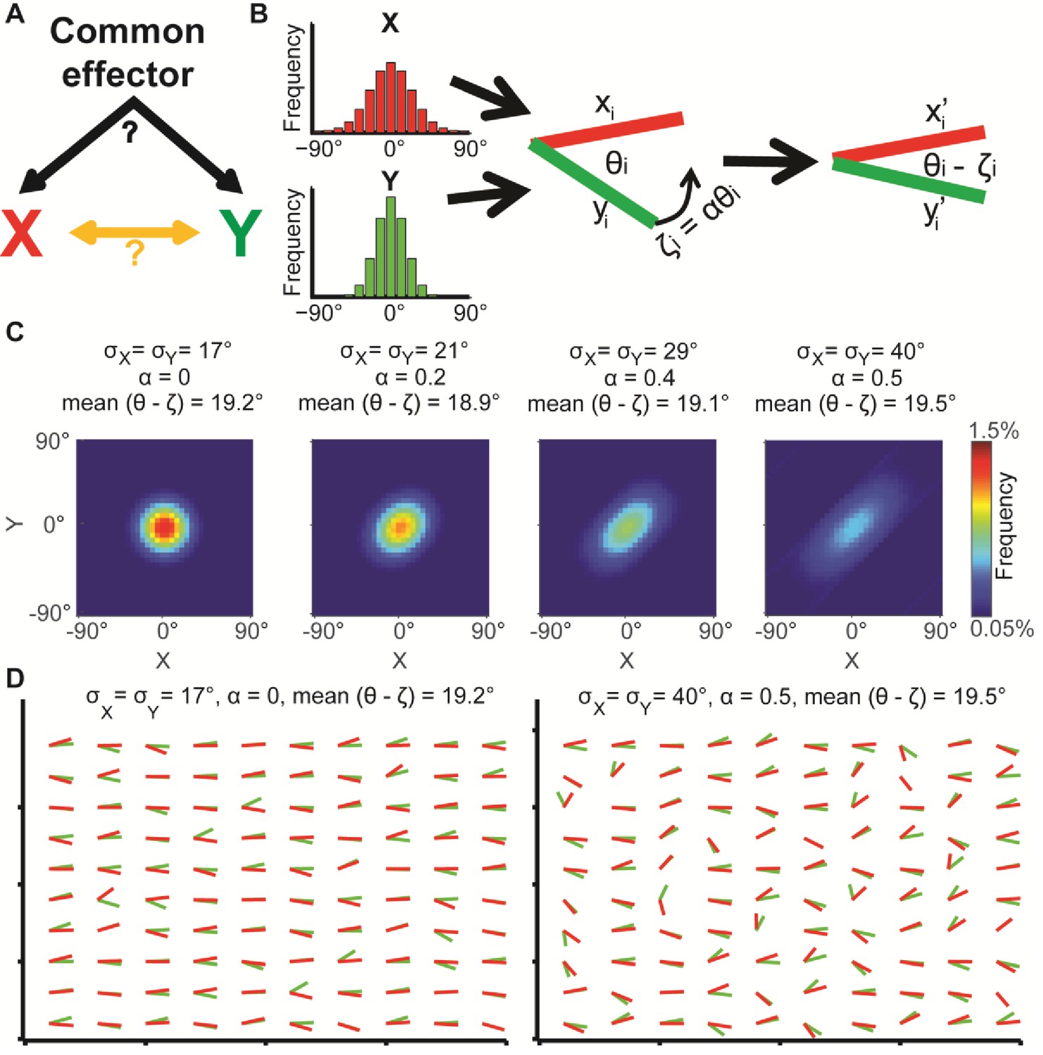
Illustration of global bias and local interaction using the alignment of two orientational variables.
(A) The relation between two variables X, Y can be explained from a combination of direct interactions (orange) and a common effector. (B) Simulation. Given two distributions X, Y, pairs of coupled variables are constructed by drawing sample pairs (xi,yi) and transforming them to (xi’,yi’) by a correction parameter ζi = αθi, which represents the effect of a local interaction. α is constant for each of these simulations. (C) Simulated joint distributions. X, Y truncated normal distributions with mean 0 and σX = σY. Shown are the joint distributions of 4 simulations with reduced global bias (i.e., increased standard deviation σX, σY) and increased local interaction (left-to-right). All scenarios have similar observed mean alignment of ~19°. (D) Example of 100 draws of coupled orientational variables from the two most extreme scenarios in panel C. Most orientations are aligned with the x-axis when the global bias is high and no local interaction exists (left), while the orientations are less aligned with the x-axis but maintain the mean alignment between (xi’,yi’) pairs for reduced global bias and increased local interaction (right).
Figure 2 with 1 supplement
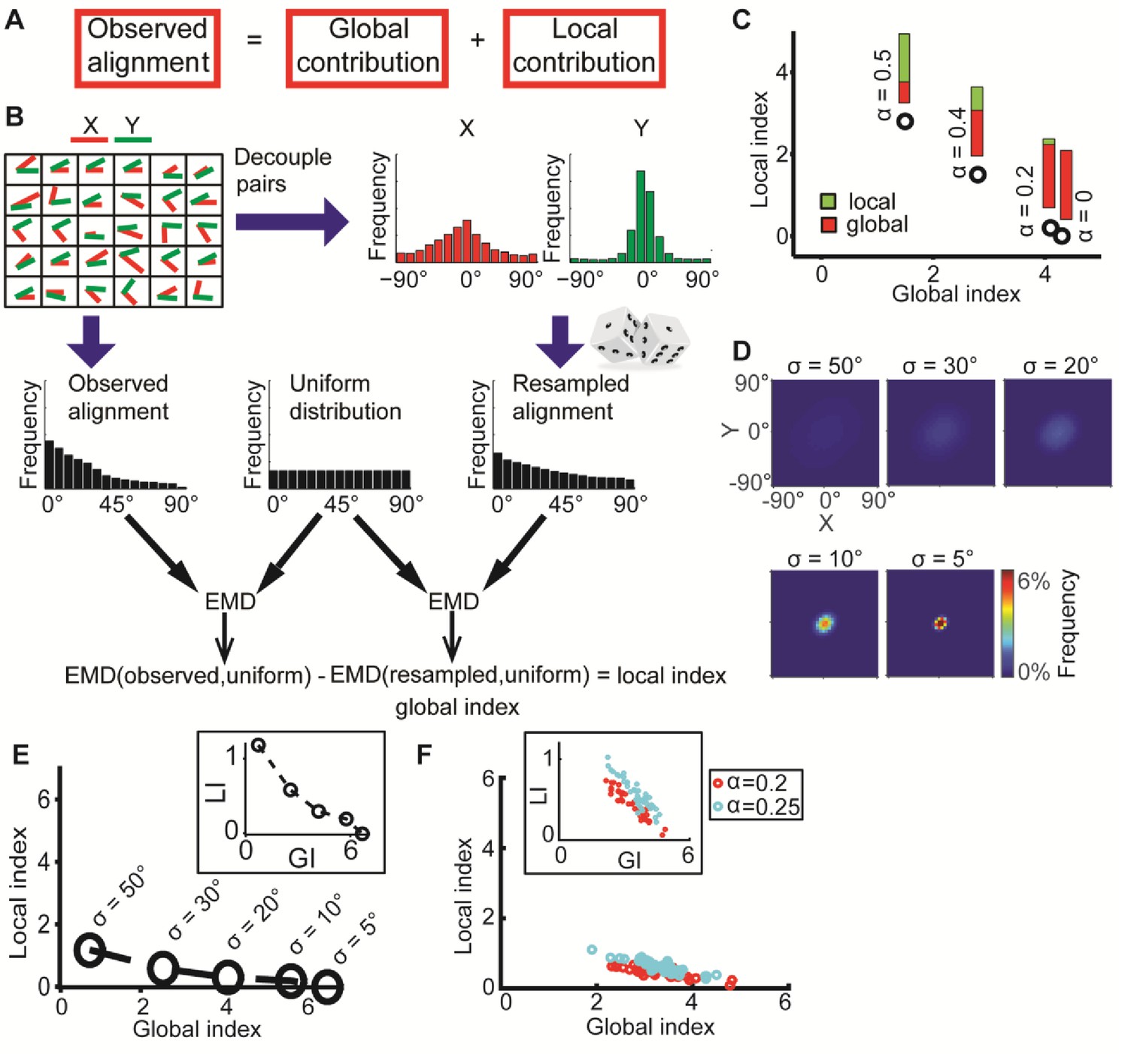
DeBias algorithm.
(A) Underlying assumption: the observed relation between two variables is a cumulative process of a global bias and a local interaction component. (B) Quantifying local and global indices: sample from the marginal distributions X, Y to construct the resampled distribution. The global index (GI) is calculated as the Earth Movers Distance (EMD) between the uniform and the resampled distributions. The local index (LI) is calculated as the subtraction of the GI from the EMD between the uniform and the observed distribution. (C) Local and global indices calculated for the examples from Figure 1C. Black circles represent the (GI,LI) value for the corresponding example in Figure 1C, bars represent the relative contribution of the local (green) and global (red) index to the observed alignment. (D-E) Simulation using a constant interaction parameter α = 0.2 and varying standard deviations of X, Y, σ = 50° to 5°. (D) Joint distributions. Correlation between X and Y is (subjectively) becoming less obvious for increasing global bias (decreasing σ). (E) GI and LI are negatively correlated: decreased σ enhances GI and reduces LI. The change in GI is ~4 fold larger compared to the change in LI indicating that the GI has a limited effect on LI values. Inset: stretched LI emphasizes the negative correlation. (F) Both LI and GI are needed to discriminate between simulations with different interaction parameters. α = 0.2 (red) or 0.25 (cyan), σ is drawn from a normal distribution (mean = 25°, standard deviation = 4°). Number of simulations = 40, for each parameter setting. Inset: stretched LI emphasizes the discrimination. Number of histogram bins, K = 15, for all simulations.
Figure 2—figure supplement 1
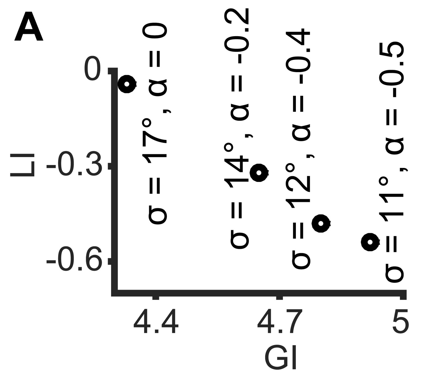
Simulations demonstrating the negative local interactions induce negative local indices.
Simulations were performed as in Figure 1B: X, Y truncated normal distributions with mean 0 and σ = σX = σY; ζ = αθ, but with α < 0 as the negative interaction. Shown are GI and LI values for four simulations with increased global bias (i.e., smaller standard deviation σX, σY) and increased negative local interaction (left-to-right), all scenarios have similar observed mean alignment of ~19° (corresponding to the simulations in Figure 1C).
Figure 3 with 1 supplement
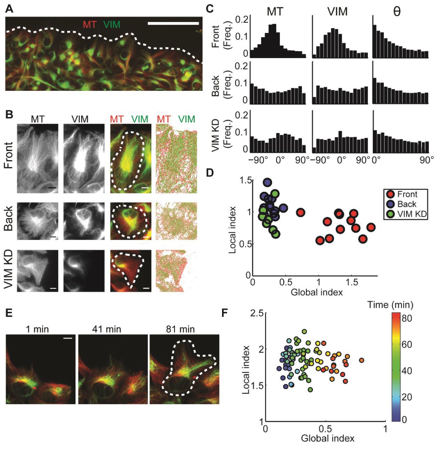
: Alignment of microtubule and vimentin intermediate filaments in the context of cell polarity.
(A) RPE cells expressing TagRFP α-tubulin (MT) and mEmerald-vimentin (VIM) at endogenous levels during a wound healing assay. Scale bar 100 μm. (B) Zooming in on cells in different locations in respect to the wound edge. Right-most column, computer segmented filaments of both cytoskeleton systems. Top row, cells located at the wound edge (‘Front’); Middle row, cells located 2–3 rows away from the wound edge (’Back’); Bottom row, cells located at the wound edge partially with shRNA knock-down of vimentin. Scale bar 10 μm. (C) Orientation distribution of microtubules (left column) and vimentin filaments (middle columns) for the cells outlined in B. Vimentin-microtubule alignment distributions (right column). (D) Scatterplot of GI versus LI derived by DeBias. The GI is significantly higher in WT cells at the wound edge (‘Front’, n = 12) compared to cells inside the monolayer (‘Back’, n = 12, fold change = 4.8, p-value < 0.0001); or compared to vimentin-depleted cells at the wound edge (‘VIM KD’, n = 7, fold change = 5.2, p-value < 0.0001). Statistics based on Wilcoxon rank-sum test. All DeBias analyses performed with K = 15. (E) Polarization of RPE cells at the wound edge at different time points after scratching. Scale bar 10 μm. (F) Representative experiment showing the progression of LI and GI as a function of time after scratching (see color code). Correlation between GI and time ~0.90, p-value < 10−30 (n time points = 83). N = 5 independent experiments were conducted of which four experiments showed a gradual increase in GI with increased observed polarity. All DeBias analyses performed with K = 15.
Figure 3—figure supplement 1
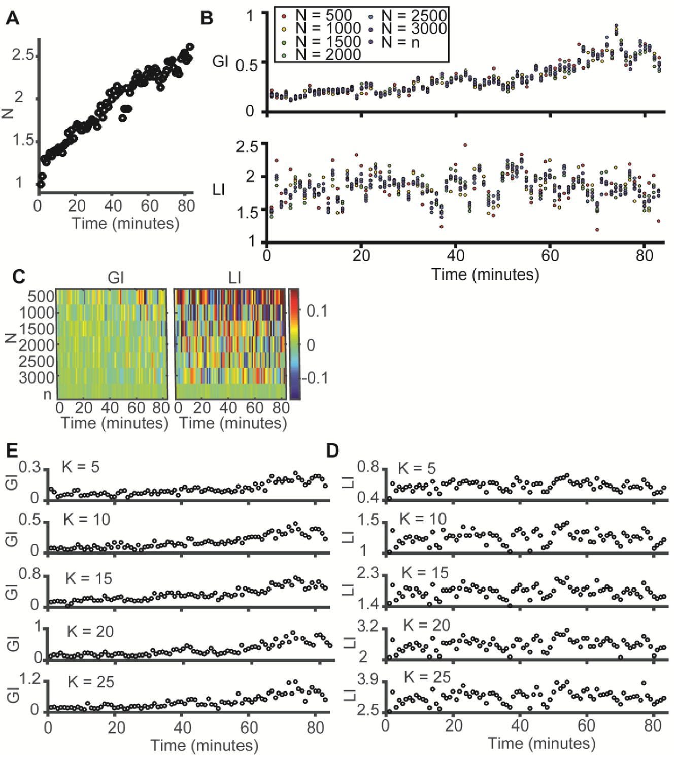
LI and GI are independent of the number of observations (N) and the number of histogram bins (K) – experimental evidence from the data in Figure 3E–F (time evolution of microtubule-vimentin alignment).
(A) Time evolution of N, the number of observations (paired microtubule and vimentin pixels) analyzed, N grows linearly in time. Y-axis was normalized to the first time point. (B–C) LI and GI are independent of the number of random resampled observations N = 500–3000. (B) LI and GI remain stable. (C) Deviation from the LI, GI values reported in Figure 3F. Lower N correspond to higher variability. All analyses performed with K = 15. (D–E) LI and GI patterns are independent of the number of alignment histogram bins K = 5–25. (D) GI. (E) LI.
Figure 4
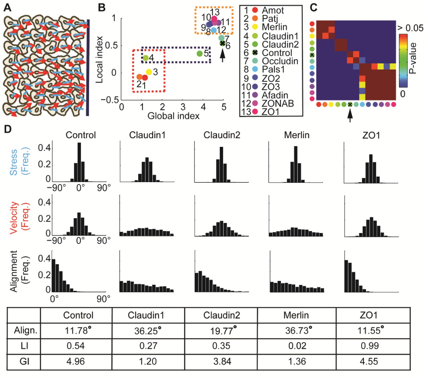
: Alignment of stress orientation and velocity direction during collective cell migration.
(A) Assay illustration. Wound healing assay of MDCK cells. Particle image velocimetry was applied to calculate velocity vectors (red) and monolayer stress microscopy to reconstruct stresses (blue). Alignment of velocity direction and stress orientation was assessed. (B) Mini-screen that includes depletion of 11 tight-junction proteins and Merlin. Data from (Das et al., 2015), where effective depletion was demonstrated. Shown are GI and LI values; molecular conditions are sorted by the LI values (control is ranked sixth, pointed by the black arrow). Each dot was calculated from accumulation of 3 independent experiments (N = 925–1539 for each condition). Three groups of tight junction proteins are highlighted by dashed rectangles: red - low LI and GI compared to control, purple – different GI but similar LI, orange – high LI. All DeBias analyses were performed with K = 15. (C) Pair-wise statistical significance for LI values. P-values were calculated via a permutation-test on the velocity and stress data (Materials and methods). Red – no significant (p ≥ 0.05) change in LI values, blue – highly significant (< 0.01) change in LI values. (D) Highlighted hits: Claudin1, Claudin2, Merlin and ZO1. Top: Distribution of stress orientation (top), velocity direction (middle) and motion-stress alignment (bottom). Bottom: table of mean alignment angle, LI and GI. Claudin1 and Claudin2 have similar mechanisms for transforming stress to aligned velocity. ZO1 depletion enhances alignment of velocity by stress.
Figure 5
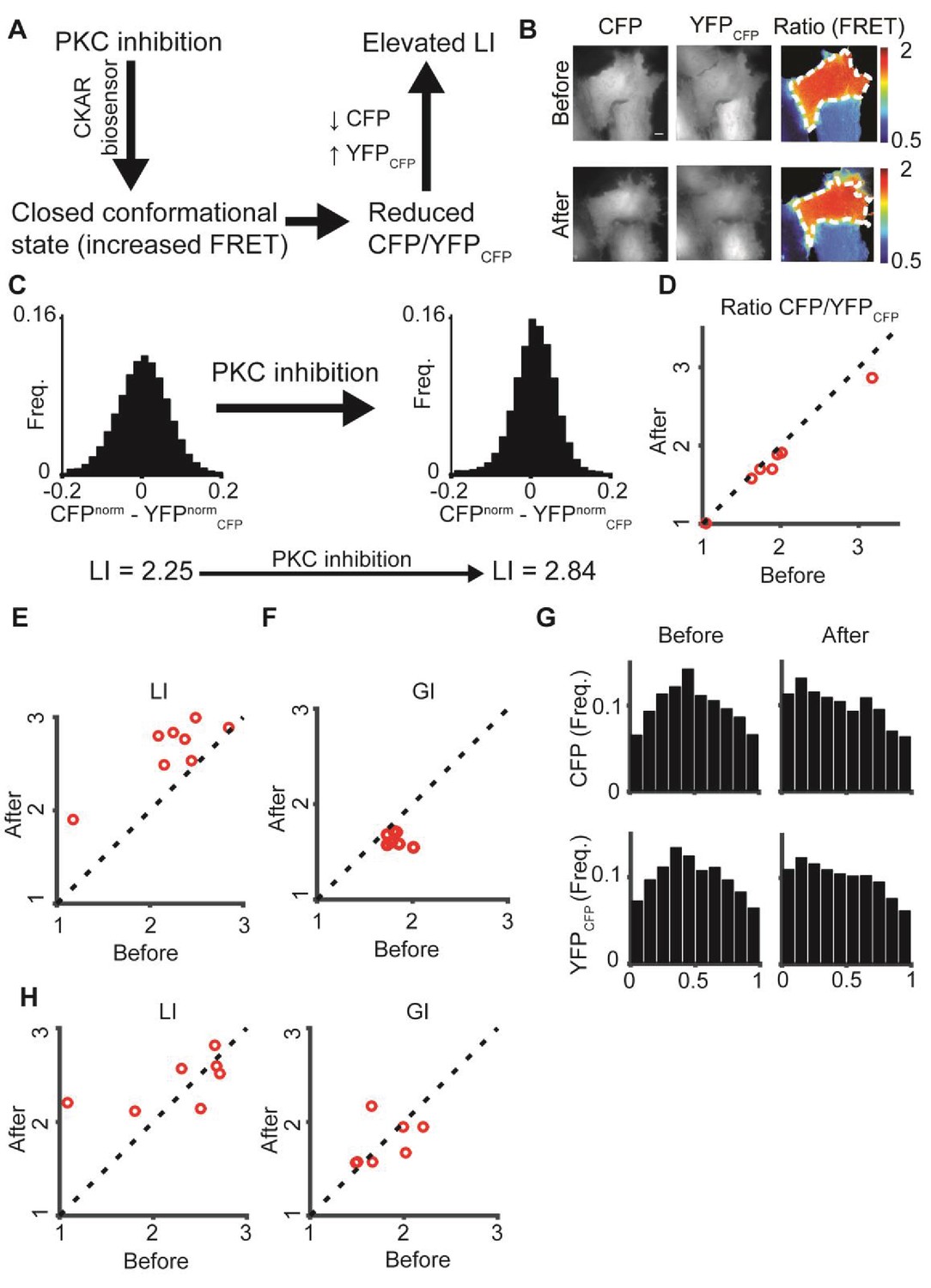
: PKC inhibition alters LI and GI.
(A) PKC inhibition is expected to lead to elevated LI for cells with dominant CFP signal (CFP > YFPCFP). Upon FRET, CFP signal is locally transferred to YFPCFP, reducing the difference in normalized intensity between the two channels, which increases LI. (B) hTERT-RPE-1 cells imaged with the CKAR reporter. A cell before (top) and after (bottom) PKC inhibition. Region of interest was manually annotated and the ratio was calculated within it. (C) Pixel distribution of differences in normalized fluorescent intensities CFPnorm - YFPnormCFP before and after PKC inhibition for the cell from panel B. PKC inhibition shifted the average absolute difference from 0.054 to 0.042 and the LI from 2.25 to 2.84. (D–F) PKC inhibition experiment. N = 8 cells. Statistics based on Wilcoxon sign-rank test. (D) The FRET ratio decreased (p-value < 0.008), (E) LI increased (p-value < 0.008), and (F) GI decreased (p-value < 0.008) after PKC inhibition. (G) Marginal distribution of CFP and YFPCFP before (top) and after (bottom) PKC inhibition. (H) Control experiment. N = 7 cells. hTERT-RPE-1 cells expressing cytoplasmic GFP and mCherry before and after PKC inhibition. No significant change in LI or GI was observed. All DeBias analyses were performed with K = 19.
Figure 6 with 1 supplement
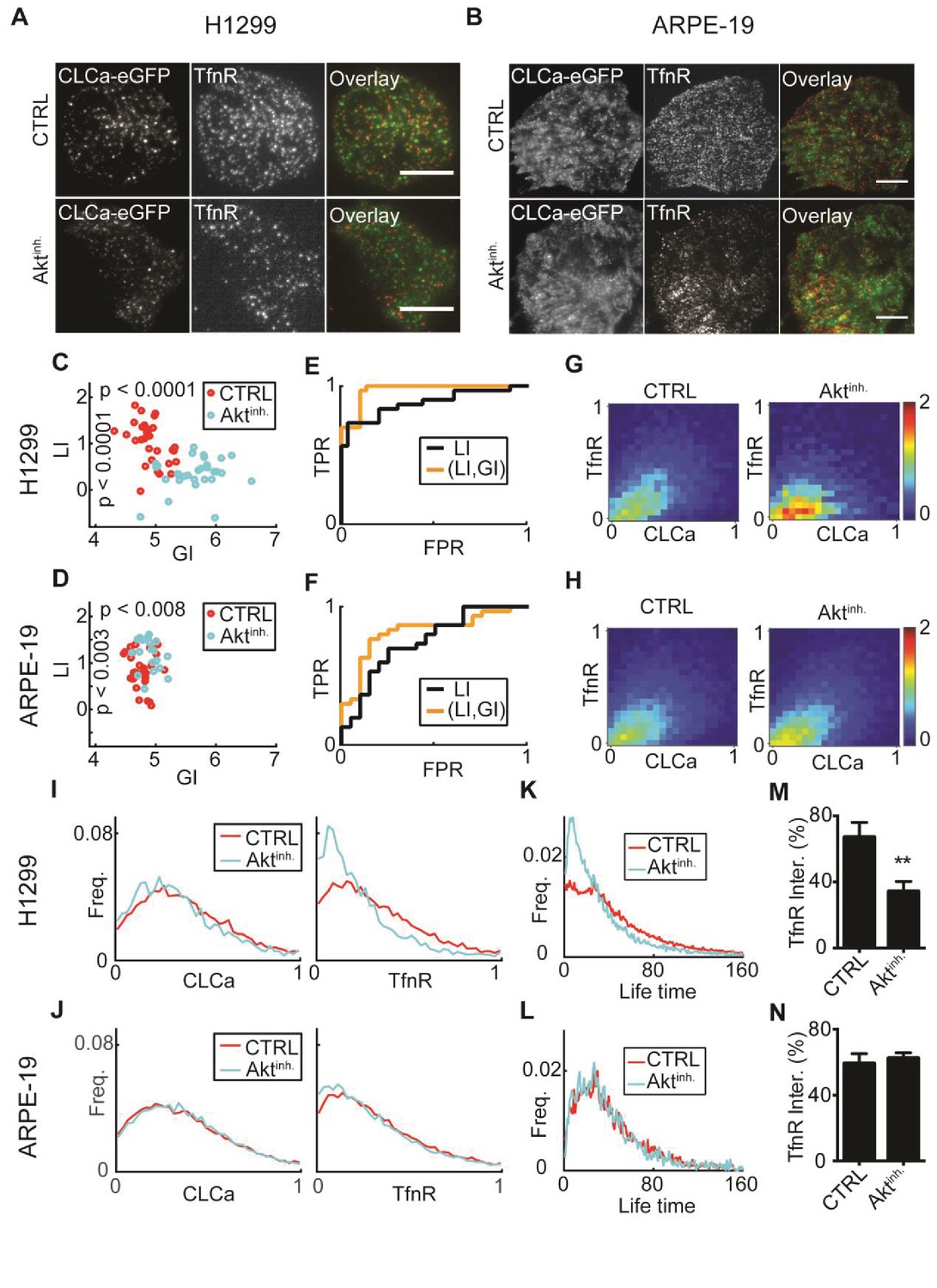
: AKT inhibition differentially alters recruitment of TfnR to CCPs during CME for different cell lines.
(A) H1299 cells expressing CLCa and TfnR ligands. Top row, representative WT cell (TfnR ligand, GI = 4.6, LI = 1.6). Bottom row, representative AKT-inhibited cell (TfnR ligand, GI = 6.0, LI = 0.3). Scale bar 10 μm. (B) ARPE-19 cells. Top row, representative WT cell (TfnR ligand, GI = 4.3, LI = 0.8). Bottom row, representative AKT-inhibited cell (TfnR ligand, GI = 4.6, LI = 1.6). (C–D) LI and GI of CLCa-TfnR co-localization for Ctrl (red) and Aktinh. cells (cyan). Every data point represents the LI and GI values for a single cell. Statistical analyses performed with the Wilcoxon rank-sum test. All DeBias analyses were performed with K = 40. (C) H1299: N number of cells Ctrl = 30, Aktinh. = 30; number of CCPs per cell: Ctrl = 455.5, Aktinh. = 179.5. GI p-value < 0.0001, LI p-value < 0.0001. (D) ARPE-19: N number of cells Ctrl = 30, Aktinh. = 20; number of CCPs per cell: Ctrl = 958.8, Aktinh. = 1138.2. GI p-value < 0.002, LI p-value < 0.008. (E–F) Receiver Operating Characteristic (ROC) curves showing the true positive rates as a function of false-positive rates for single cell classification, higher curves correspond to enhanced discrimination (Materials and methods). Black – LI, orange – (GI,LI). Statistics via permutation test (Materials and methods). (E) H1299 AUC: (GI,LI) = 0.96 versus LI = 0.88, p-value ≤ 0.003. (F) ARPE-19 AUC: (GI,LI) = 0.83 versus LI = 0.72, p-value ≤ 0.048. (G–H) Joint distributions of CLCa (x-axis) and TfnR (y-axis) for H1299 (G) and ARPE-19 (H) cells. (I–J) Marginal distributions of CLCa (left) and TfnR (right) for H1299 (I) and ARPE-19 (J) cells. (K–L) Combined CCP lifetime distribution for 50 Ctrl (red) and Aktinh. (cyan) cells. Statistics with Wilcoxon rank-sum test (Materials and methods). (K) H1299: p-value < 0.006 (mean EMD: Ctrl = 29.3 versus Aktinh. = 43.6); number of cells: 50 (Ctrl), 11 (Aktinh.). (L) H1299: p-value n.s. (mean EMD: Ctrl = 36.1 versus Aktinh. = 38.0); number of cells: 12 (Ctrl), 12 (Aktinh.). (M–N) Percentage of TfnR uptake: Ctrl versus Aktinh. (whiskers - standard deviation). Statistics via two-tailed Student’s t-test. (M) H1299: p-value < 0.005; N = 3 independent experiments. (N) ARPE-19: p-value n.s.; N = 3 independent experiments.
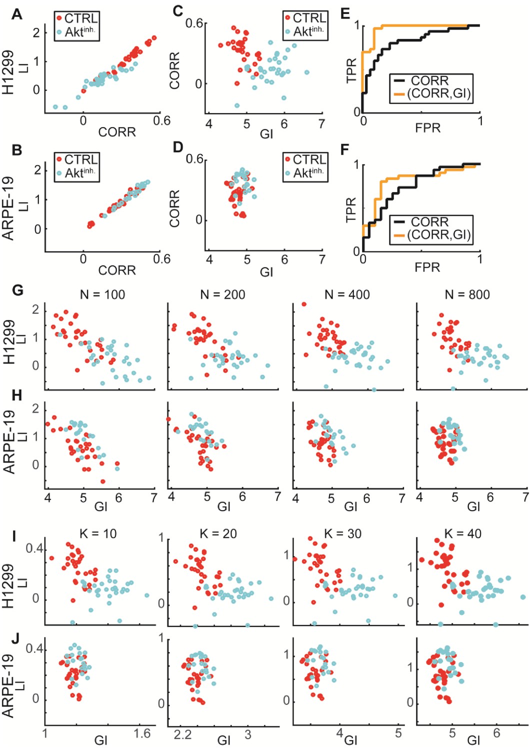
Figure 6—figure supplement 1
: GI encodes information that is distinct from local interactions; Experimental validations of DeBias for co-localization.
Data from Figure 6. (A–F) GI as a complementary measure. (A–B) LI and Pearson’s correlation (CORR) are highly associated (statistical analyses performed using Pearson’s correlation). (A) H1299 cells: rho = 0.95, p-value < 10−29. (B) ARPE-19 cells: rho = 0.98, p-value < 10−32. (C–D) CORR vs. GI. (C) H1299. (D) ARPE-19. (E–F) ROC curves. Statistics via permutation test (Materials and methods). (E) H1299 AUC: (GI,CORR) = 0.96 versus CORR = 0.83, p-value ≤ 0.0001. (F) ARPE-19 AUC: (GI,CORR) = 0.84 versus CORR = 0.72, p-value n.s.. (G–H) Similar LI, GI values for different number of observations N = 100, 200, 400, 800. (G) H1299. (H) ARPE-19. (I–J) LI and GI patterns are independent of the number of alignment histogram bins K = 10, 20, 30, 40. (I) H1299. (J) ARPE-19.
Appendix 2—figure 1
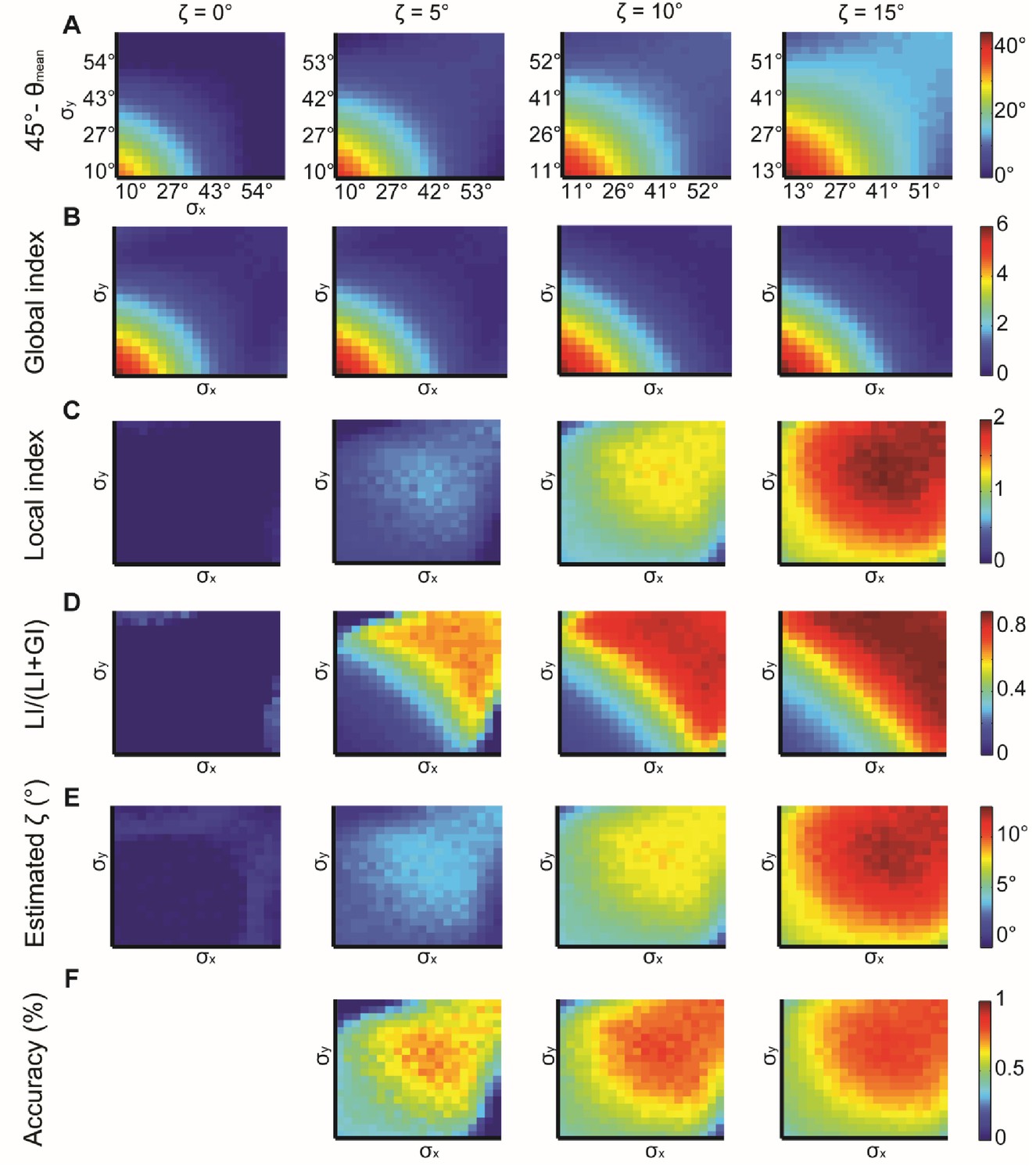
Simulations for X, Y normal distributions with different x, y and constant ζ = 0°, 5°, 10°, 15°.
(A) 45° – θmean reflecting the cumulative effect of the global bias and the local interaction between X, Y (θmean is the mean observed alignment). Lower variance and higher correspond to better alignment. (B) Global index. has a small effect on GI. (C) Local index. has a major effect on LI. (D) Relative contribution of LI to the observed alignment increases as function of ζ. (E) Retrieved estimated calculated as the relative contribution of LI to the observed alignment (panel D) times the cumulative effect of the global bias and the local interaction (panel A). (F) Accuracy of estimated grows with and with lower x, y. Note, that this estimation is a lower bound for the true (Appendix 1, Theorem 4). Accuracy cannot be measured for = 0° hence the empty panel.
Appendix 2—figure 2
Simulations for different values of K, the number of bins in the alignment distribution.
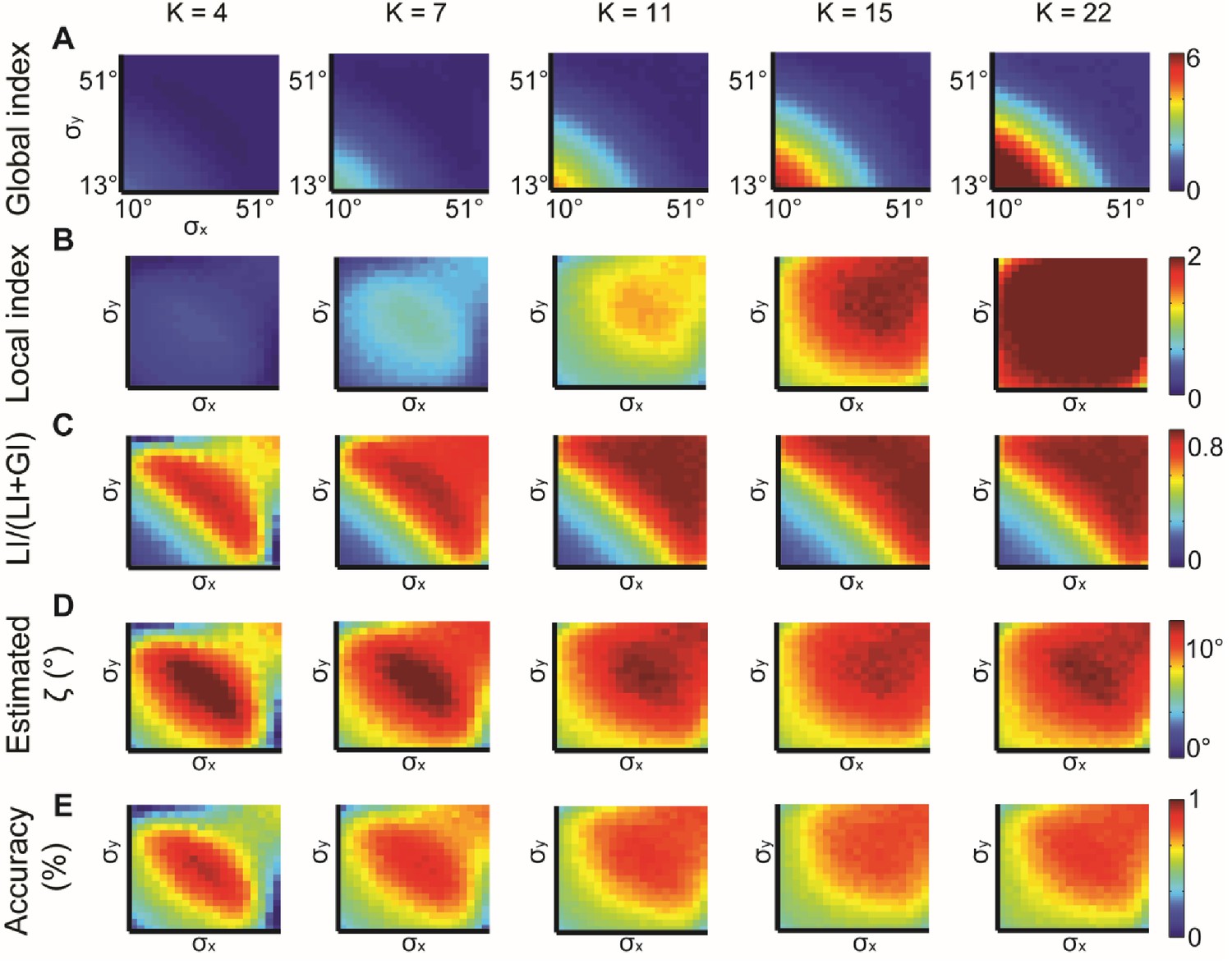
normal distributions with different and constant ζ = 15°. K = 4, 7, 11, 15, 22 were examined. (A–B) Global (A) and local (B) indices grow with K. (C–E) Relative contribution of LI to the observed alignment (C), Retrieved estimated (D) and accuracy of estimated (E) stabilizes for K ≥ 11.
Appendix 2—figure 3
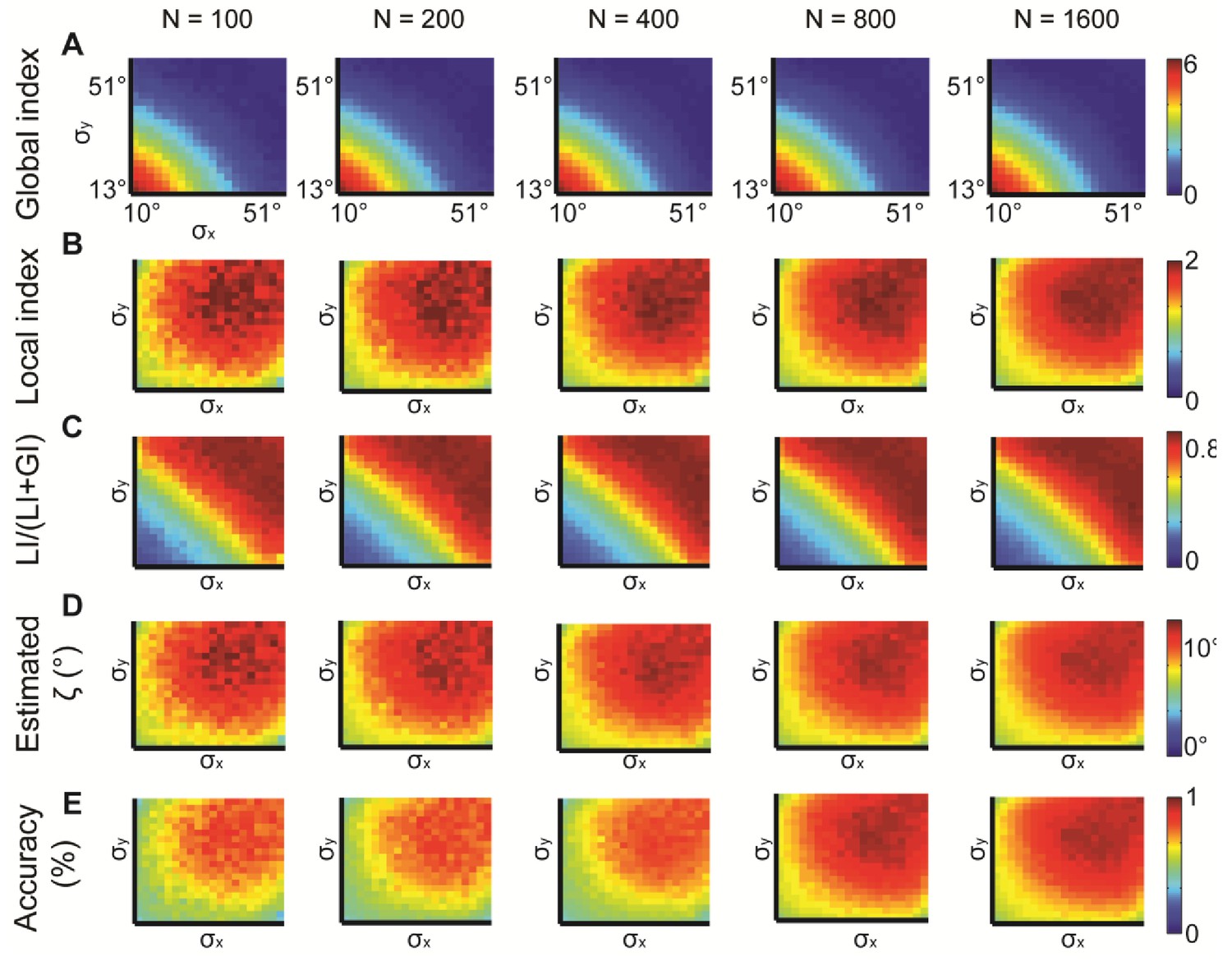
Simulations for different N, the number of observations.
N = 100, 200, 400, 800, 1600 were examined. normal distributions with different and constant = 15°. All measures provide similar information but are noisier for lower N. (A) Global index. (B) Local index. (C) Relative contribution of LI to the observed alignment. (D) Retrieved estimated ζ. (E) Accuracy of estimated ζ.
Appendix 3—figure 1
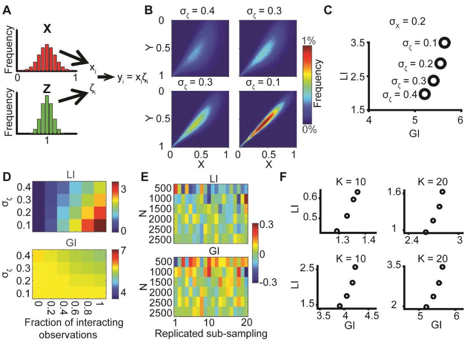
Simulating co-localization.
(A) Simulation. We use the distributions , where X is truncated to [0,1]. Pairs of coupled variables are constructed by drawing sample pairs () and constructing (Materials and methods). (B) Simulated joint distributions. Shown are the joint distributions of 4 simulations with increased global bias (i.e., decreased ). (C) Local and global indices calculated for the examples from panel B. Smaller associate with larger LI. The weaker negative association between GI and is because larger induces a distribution that is more spread compared to which reduces the GI. (D) Simulations of partial co-localization. A given fraction of observations for were calculated as shown in panels A–C, the rest were independently drawn from the distribution implying no local interaction. Shown are LI (top) and GI (bottom) as functions of the fraction of locally interacting observations and . LI associates with increased fraction of locally-interacting observations, whereas the effect is minor in GI, in accordance with panel C. (E) Deviation of LI, GI values reported in panel C as functions of the number of observations n. 20 independent sub-sampling. Lower n associates with higher variability. No other trend is observed. (F) LI and GI patterns are independent of the number of alignment histogram bins K = 10–40. Equal size of dynamic ranges was set for LI and GI plots in panels C, D and F. K, number of histogram bins was set to 40 for all panels excluding F. = 0.2 for panels B–E.
Author response image 1

Videos
Video 1
Polarization of RPE cells at the monolayer edge over time.
Please note several occasions (44 and 46 min, 65 and 67 min, 73 and 75 min) of focus drift followed by automated focus correction.
Tables
Appendix 4 – Table 1
Object- versus pixel-based colocalization.
Object-based methods are best applicable for the colocalization of binary signals, but not/less for applications, in which colocalization accounts for coupling of molecular counts on a continuous spectrum.
| Pixel based | Object based |
|---|---|
| Pixel-wise correlation | Spatial colocalization |
| Limited to object-detectable data | |
| Suffer from background signal | |
| Highly altered by detection accuracy | |
| Affected by confounding factors (e.g., CCP size) | Lose the information at the detected objects |
Download links
A two-part list of links to download the article, or parts of the article, in various formats.
Downloads (link to download the article as PDF)
Open citations (links to open the citations from this article in various online reference manager services)
Cite this article (links to download the citations from this article in formats compatible with various reference manager tools)
Decoupling global biases and local interactions between cell biological variables
eLife 6:e22323.
https://doi.org/10.7554/eLife.22323


