UP-DOWN cortical dynamics reflect state transitions in a bistable network
Figures
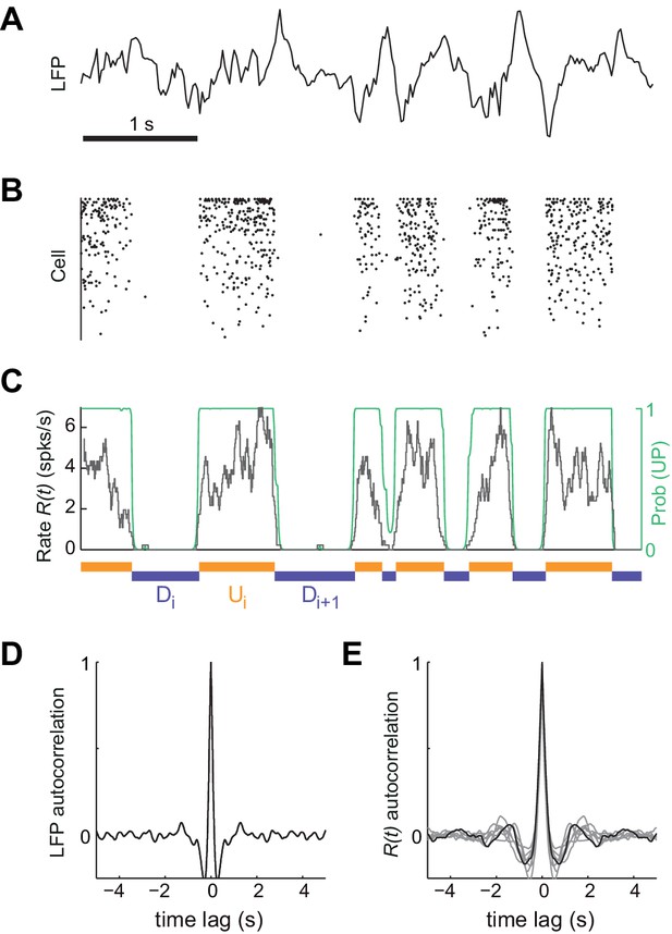
Synchronized brain activity under urethane anesthesia in the rat somatosensory cortex and the detection of putative UP and DOWN periods.
(A) Local field potential during 5 s of synchronized state displaying high-amplitude slow fluctuations. (B) Population raster of 92 simultaneously recorded single units exhibiting the alternation between periods of tonic spiking activity and periods of neural quiescence (cells sorted based on mean firing rate). (C) Instantaneous population rate (grey) is used to identify putative U (orange) and D (purple) periods. The detection algorithm is based on fitting a Hidden Markov Model (HMM) and computing the posterior probability of the hidden state being in an UP state (green) (see Materials and methods). (D) Average autocorrelogram of LFP (20 s windows) for one example experiment. (E) Average autocorrelogram of R(t) for different (n = 7) experiments (example experiment in black).
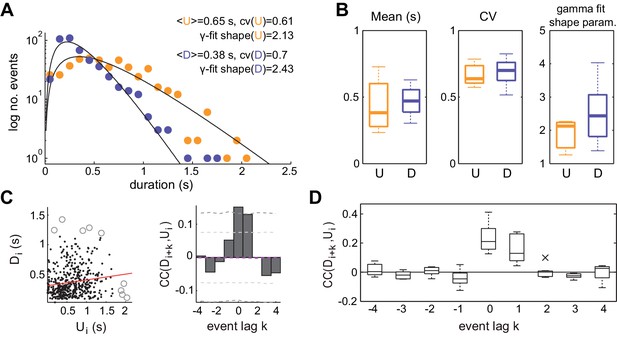
Statistics of U and D periods during synchronized brain activity.
(A) Distribution of U and D durations for one example experiment (same as Figure 1). Inset shows the mean and coefficient of variation (CV) of U and D durations. (B) Summary of period duration mean (left), CV (middle), and gamma-fit shape parameter (right) across experiments (n = 7 rats). While average durations are quite heterogeneous across experiments, the period duration variability is consistently large. (C) Left: D duration (Di) vs the consecutive U duration (Ui) exhibit weak but significant serial correlation. Values more than 3 standard deviations away from the mean (circles) were discarded for correlation analysis. Red line shows linear regression. Right: Cross-correlogram between the Di and Ui sequences for different lags (k) in a single experiment. Magenta dashed line represent the mean cross-correlogram from a local shuffled (see Materials and methods). Light (dark) grey dashed line showing 95% C.I. point-wise (global) error bands. (D) Summary of cross-correlation analysis for the different experiments, displaying consistent positive correlations across experiments for lags k = 0 and k = 1.
-
Figure 2—source data 1
U and D period durations and statistics for individual experiments.
- https://doi.org/10.7554/eLife.22425.005
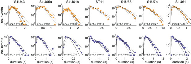
Distributions of U and D period durations for individual experiments.
Distributions of U (top row) and D (bottom row) period durations for the seven experiments (columns). Gamma fit for each distribution is shown in black. The shape a and scale b parameters of the Gamma fit are displayed at the bottom of each panel. 95% CI of the fit displayed in dashed line.
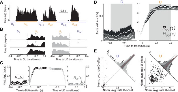
Population spiking statistics during U and D periods.
(A) Example of instantaneous population rate with U and D detected periods (as in Figure 1). (B–C) Each U period is aligned at the DU (B, left) and UD (B, right) transition times in order to compute the instantaneous population rate averaged across transitions (C, dark grey) and (C, light grey), respectively. Only periods longer than 0.5 s (asterisks in B) were included in the average. (D) Comparison of population rate at the onset and offset of Us and Ds done by overlaying and a time-reversed . Onset and offset windows defined during D and U periods (shaded) were used to test significance of changes in the rate. (E) Normalized firing rates from all individual neurons (448 cells from n = 7 animals) during onset and offset windows. Left: D periods. Right: U periods. Average across cells is shown in red. Gray bands show 95% C.I. of the histograms obtained from onset-offset shuffled data (see Materials and methods).
-
Figure 3—source data 1
Instantaneous population rate averaged across transitions and for individual experiments.
- https://doi.org/10.7554/eLife.22425.008

Firing rate statistics for single units during U and D periods.
(A) Scatter plot of average firing rate during U periods versus firing rate during D periods (RU vs RD), from all the isolated cells from the different experiments (n = 7 animals; 448 cells). Marginal distribution of firing rates for RU in orange and RD in purple. (B) Statistics of mean single cell firing rates during D (left boxplot) and U (right boxplot) periods for different experiments. (C) Statistics of mean correlation between firing rate during D and U periods for different experiments.
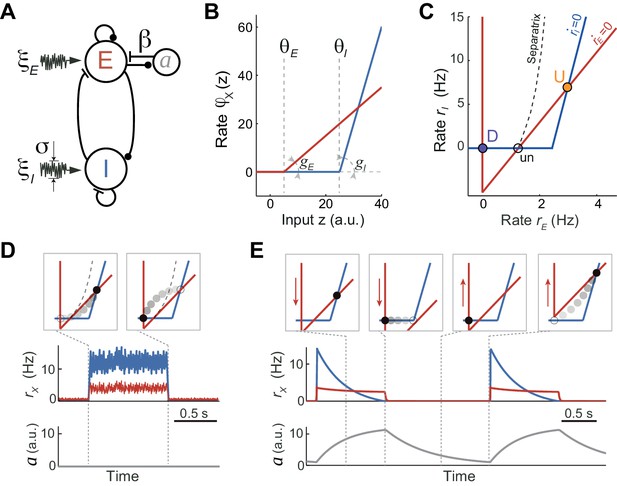
Rate model for fluctuations and adaptation induced UP and DOWN dynamics.
(A) Network composed of recurrently connected inhibitory (I, blue) and excitatory (E, red) populations, with E exhibiting rate adaptation a(t) and both populations receiving independent fluctuating external inputs. (B) Transfer functions for the E and I populations are threshold-linear with unequal thresholds θE < θI and unequal gains gE < gI. This marked asymmetry is at the origin of the bistability obtained in the network. (C) In the absence of adaptation, the phase plane of rates rE vs. rI shows the E and I nullclines (red and blue, respectively) whose intersections determine two stable (U and D) and one unstable (un) fixed points. The separatrix (dashed line) divides the phase plane into the basins of attraction of the D and U stable points. (D, E) Schematics of fluctuations-induced DU and UD transitions in the absence of adaptation (β = 0) and adaptation-induced transitions in the absence of fluctuations (σ = 0), respectively. Traces of rE(t), rI(t) and adaptation a(t) illustrate steady fluctuating rates during U periods when there is no adaptation (D), and a periodic alternation between U and D characterized by a strongly decaying I rate during Us when there is no fluctuations (E). Top insets show the network trajectories in the phase-plane taken at different time points (vertical dotted lines). Notice the downward (upward) displacement of the E-nullcline during U (D) periods (red arrows in E). Connectivity parameters: JEE = 5, JEI = 1, JIE = 10, JII = 0.5 s; Transfer function parameters: gE = 1, gI = 4 Hz, θE = 0, θI = 25 a.u.
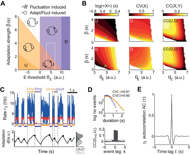
Fluctuations and weak adaptation are required in the model to explain the U-D statistics of the data.
(A) Different dynamical regimes of the model as a function of the adaptation strength β and the effective threshold θE. Each U and D state is either meta-stable or quasi-stable depending on whether the transitions to the opposite state can be caused by fluctuations or adaptation + fluctuations, respectively (see arrow code in top inset). There are five region types: regions with a single stable state and no transitions (dark purple and dark orange), a region with both U and D meta-stable (light red), one with both U and D quasi-stable (white) and mixed regions with a meta-stable and a quasi-stable state (light orange and light purple). (B) Statistics of U (top) and D (bottom) periods obtained from numerical simulations: mean durations (left), duration CV (center) and of cross-correlation CC of consecutive periods (right) as a function of β and θE. The region analyzed is marked in A (gray rectangle). Fluctuations were σ = 3.5. White areas indicate very low transition rate. (C–E) Model example quantitatively reproducing some U-D statistics of the data. The β and θE used are marked in B (green square; θE = 4.8 a.u., β = 0.7 Hz−1). Example traces of rE(t), rI(t), and (t) show U-D transitions with irregular durations (C). Black and gray filled dots indicate the adaptation values at the UD and DU transition times, respectively. The corresponding histograms illustrate the variability of these values (C bottom right). (D) Top: Distributions of U and D period durations. Bottom: Cross-correlograms of D and U periods for different lag values (compare with Figure 2C). Grey dashed lines show global error bands and magenta dashed line shows mean CC of shuffles. (E) Autocorrelogram of rE(t) shows no traces of rhythmicity.
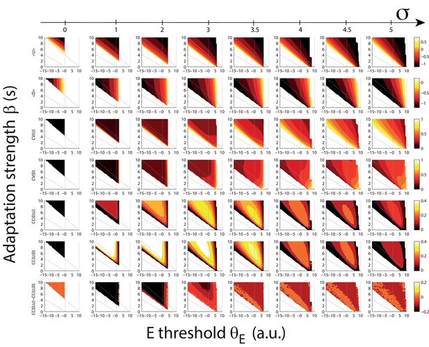
Statistics of U and D durations as a function of the adaptation strength β and the effective threshold θE for different amplitude of fluctuating external inputs.
From top to bottom: mean U, mean D, CV of U, CV of D, cross-correlation (CC) of consecutive DU periods, CC of consecutive UD periods, difference between CC of consecutive DU and UD periods. Different columns represent increasing values of the standard deviation of the fluctuating external inputs (see upper scale bar). Grey lines define the different dynamical regimes of the model in the absence of fluctuations (as in Figure 5A).
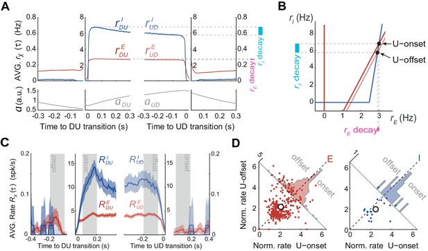
Excitatory and inhibitory populations during UP and DOWN alternation dynamics.
(A) Model average population rates rE and rI and adaptation a as a function of time, aligned at DU and UD transitions (same simulation parameters as in Figure 5C). (B) Model predicts a pronounced decay for rI (cyan bar) with minimal decay of rE (pink bar) throughout UP periods, despite adaptation is exclusively included in E cells (Figure 4A). (C) Example experiment averaged putative excitatory and inhibitory population rates (RE(τ) and RI(τ), respectively) aligned at DU and UD transitions. (D) Normalized firing rates from individual neurons (see Materials and methods) pooled from different experiments (n = 5; 330 putative E cells and 21 putative I cells active during U) comparing the activity from putative E and I cells during U onset and offset periods (gray shaded areas from panel C), reveals a significant decrease of I cells during U periods.
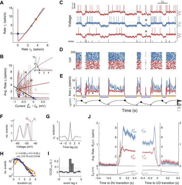
UP and DOWN dynamics in an EI network model of spiking neurons.
(A) Phase plane of population averaged rates rE vs. rI showing the E and I nullclines (red and blue, respectively) obtained using mean-field expressions for the rates. The E nullcline is drawn twice assuming an AHP current fixed at the mean value observed at the UP onset (dark red) and offset (light red). Filled circles display UP (orange) and DOWN (purple) stable fixed points for each case. (B) Bifurcation diagram showing the stable (solid) and unstable (dashed) fixed points of the rates rE (red) and rI (blue) as a function of the difference between the external current and . The straight line shows the dependence of the AHP current at equilibrium with the rate rE. Solid dots show fixed stable points of the system. Superimposed (rE, ) trace shows a 10 s example of UP to DOWN transitions obtained from simulations (also shown in C-E). Arrowheads mark the point in this trace where DU (orange) and UD (purple) transitions were detected. Note the considerable variance along the axes for the two sets of arrowheads, required to produce serial correlations. Inset shows a zoom-out of this plot where the two bifurcation points (saddle-nodes) are visible. (C–E) Network activity snapshot (duration 10 s) showing the membrane voltage of three example I (blue) and E (red) neurons (only the neuron in the top receives kicks), train of external kicks (tick size represents kick amplitude) (C), spike rastergram of 100 E and 100 I cells (D), population averaged rates rE(t) vs. rI(t) (E top) and population averaged AHP current (t) (E bottom). Orange and purple horizontal lines indicate U and D intervals detected automatically as with the experimental data (compare with Figure 1). (F) Membrane voltage distributions for E and I cells (top and middle neurons shown in C). Vertical dashed lines display their spiking thresholds and . (G) Autocorrelogram of the population averaged rate rE(t). (H) Distribution of U and D durations (dots) and gamma fits (lines). Legend shows the mean and CV of U and D durations (order parameter of the fits were = 1.1;0.7 and = 2.3;0.4 - shape;scale parameters). (I) Cross-correlogram of D and U periods for different lag values (compare with Figure 2C). Light (dark) grey dashed lines show 95% C.I. point-wise (global) error bands. (J) Population averaged rates rE and rI (top) and AHP current (bottom) as a function of time, aligned at DU and UD transitions (as in Figure 6A,C).
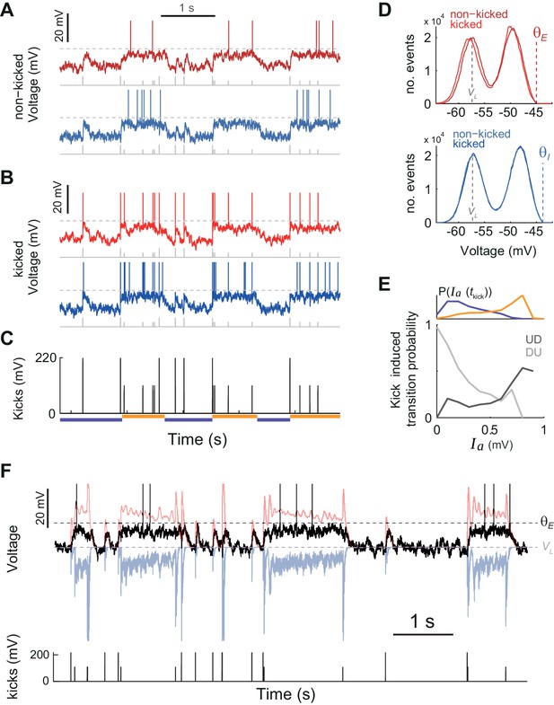
Kicks impinging on a minority of neurons induce coherent network transitions, with effectiveness depending on AHP current values.
(A) Membrane voltage for non-kicked E (top) and I (bottom) example cells (dashed lines display spiking thresholds ). Kicks received by the network are shown as bottom gray ticks. Notice that both during D and U periods, there are kicks that failed to cause a transition. (B) Membrane voltage for kicked E (top) and I (bottom) example cells. (C) Train of kicks impinging on the network. Notice that kick amplitude is lower during UP periods. Orange and purple horizontal lines indicate U and D detected intervals. (D) Membrane voltage histograms for kicked and non-kicked E (top) and I (bottom) cells. Gray and colored dashed lines display leak current VL and threshold, respectively. Notice that kicked and non-kicked neurons display completely analogous dynamics as the population coherently transitions between U and D states. (E) Top: Probability density function of at kick time taking place at D (purple) and U (orange) periods. Bottom: Kicked induced transition probability, defined as the probability of a kick causing a transition (DU in light gray, UD in dark gray) for a given value. In both types of transitions the adaptation current plays a large role modulating the effectiveness of the kicks triggering transitions. (F) The membrane voltage for a non-kicked E example cell (black) is shown simultaneously with the recurrent excitatory (, in red) and inhibitory (, in blue) synaptic inputs received by the cell. Dark and light gray dashed lines display the threshold () and leak potential (), respectively. The train of kicks received by the network is displayed below.
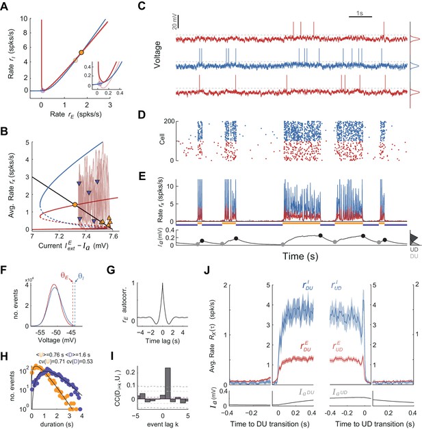
UP and DOWN dynamics in the EI spiking network model caused by independent Gaussian noise.
(A–B) Phase plane of population averaged rates rE vs. rI and bifurcation diagrams (as in Figure 7A–B). In A, Inset displays zoom-in area for the D fixed point. Although U-D transitions can take place at different points along the upper branch of the bifurcation diagram, D-U transitions take place only close at the lower saddle-node point (i.e. the knee) where the DOWN state loses stability (compare horizontal scatter of purple and orange arrowheads). (C–E) Example of 10 s network activity snapshot with the membrane voltage of three example neurons (in blue I cell, in red E cells) (C), spike rastergram of 100 E and 100 I cells (D), population averaged rates rE(t) vs. rI(t) (E top) and population averaged AHP current (E bottom). (F) Membrane voltage distributions for E and I example cells are unimodal (top and middle neurons shown in C). Vertical dashed lines display spiking thresholds. (G) Autocorrelogram of the population averaged rate rE(t). (H) Distribution of U and D durations (dots) and gamma fits (lines). Inset shows the mean and CV of U and D durations (order parameter of the fits were = 1.9;0.4 and = 3.2;0.5 - shape;scale parameters). (I) Cross-correlogram of D and U periods for different lag values (compare with Figures 2C and 7I). Light (dark) grey dashed lines show 95% C.I. point-wise (global) error bands. Although correlations between consecutive U-D periods are preserved in this case, correlations between consecutive D-U periods are vanished. (J) Average population rates rE and rI as a function of time, aligned at DU and UD transitions (as in Figure 7J).
Additional files
-
Transparent reporting form
- https://doi.org/10.7554/eLife.22425.016


