Towards deep learning with segregated dendrites
- University of Toronto Scarborough, Canada
- University of Toronto, Canada
- DeepMind, United Kingdom
- Canadian Institute for Advanced Research, Canada
Figures
Figure 1
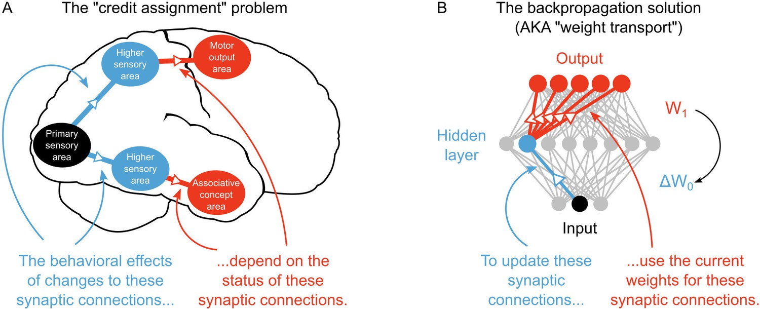
The credit assignment problem in multi-layer neural networks.
(A) Illustration of the credit assignment problem. In order to take full advantage of the multi-circuit architecture of the neocortex when learning, synapses in earlier processing stages (blue connections) must somehow receive ‘credit’ for their impact on behavior or cognition. However, the credit due to any given synapse early in a processing pathway depends on the downstream synaptic connections that link the early pathway to later computations (red connections). (B) Illustration of weight transport in backpropagation. To solve the credit assignment problem, the backpropagation of error algorithm explicitly calculates the credit due to each synapse in the hidden layer by using the downstream synaptic weights when calculating the hidden layer weight changes. This solution works well in AI applications, but is unlikely to occur in the real brain.
Figure 2
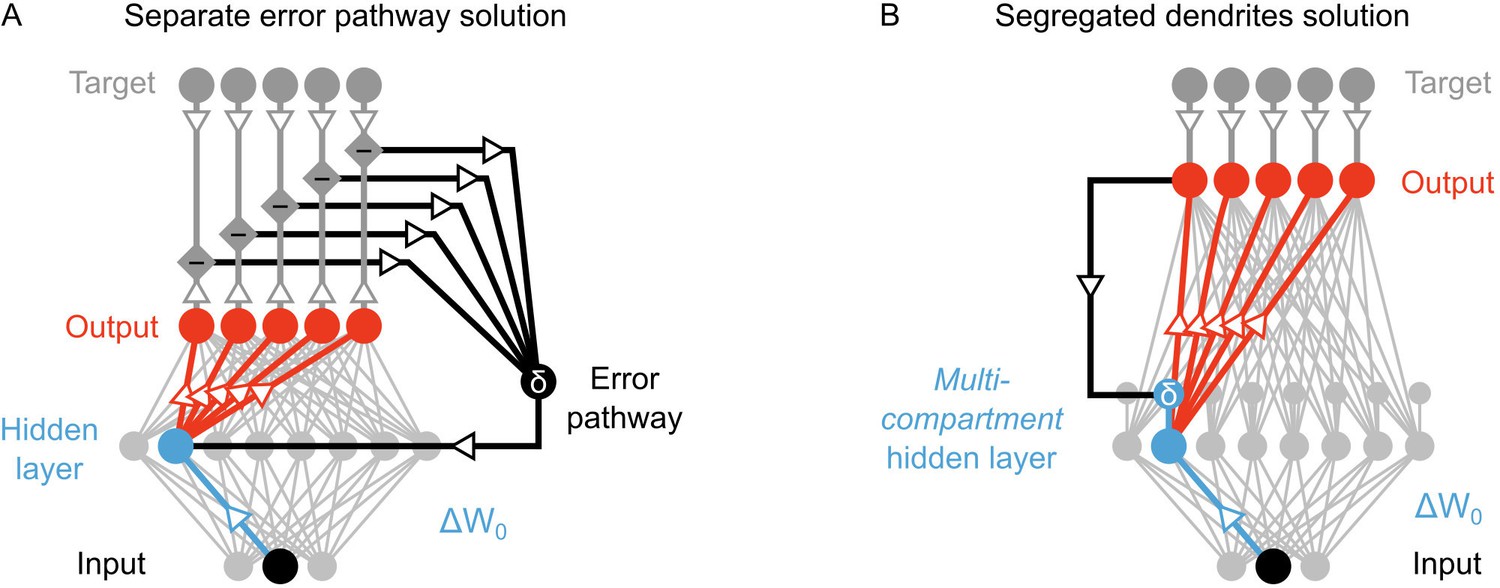
Potential solutions to credit assignment using top-down feedback.
(A) Illustration of the implicit feedback pathway used in previous models of deep learning. In order to assign credit, feedforward information must be integrated separately from any feedback signals used to calculate error for synaptic updates (the error is indicated here with ). (B) Illustration of the segregated dendrites proposal. Rather than using a separate pathway to calculate error based on feedback, segregated dendritic compartments could receive feedback and calculate the error signals locally.
Figure 3
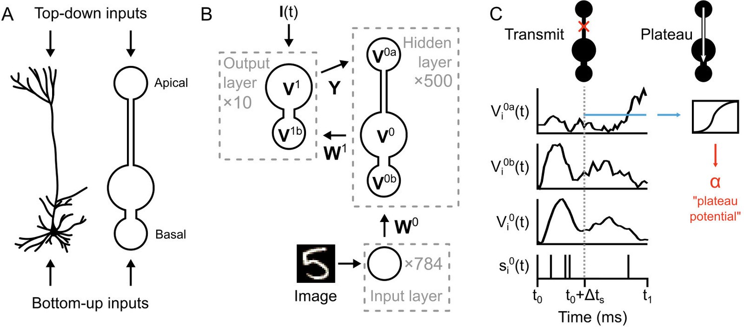
Illustration of a multi-compartment neural network model for deep learning.
(A) Left: Reconstruction of a real pyramidal neuron from layer five mouse primary visual cortex. Right: Illustration of our simplified pyramidal neuron model. The model consists of a somatic compartment, plus two distinct dendritic compartments (apical and basal). As in real pyramidal neurons, top-down inputs project to the apical compartment while bottom-up inputs project to the basal compartment. (B) Diagram of network architecture. An image is used to drive spiking input units which project to the hidden layer basal compartments through weights . Hidden layer somata project to the output layer dendritic compartment through weights . Feedback from the output layer somata is sent back to the hidden layer apical compartments through weights . The variables for the voltages in each of the compartments are shown. The number of neurons used in each layer is shown in gray. (C) Illustration of transmit vs. plateau computations. Left: In the transmit computation, the network dynamics are updated at each time-step, and the apical dendrite is segregated by a low value for , making the network effectively feed-forward. Here, the voltages of each of the compartments are shown for one run of the network. The spiking output of the soma is also shown. Note that the somatic voltage and spiking track the basal voltage, and ignore the apical voltage. However, the apical dendrite does receive feedback, and this is used to drive its voltage. After a period of to allow for settling of the dynamics, the average apical voltage is calculated (shown here as a blue line). Right: The average apical voltage is then used to calculate an apical plateau potential, which is equal to the nonlinearity applied to the average apical voltage.
Figure 4
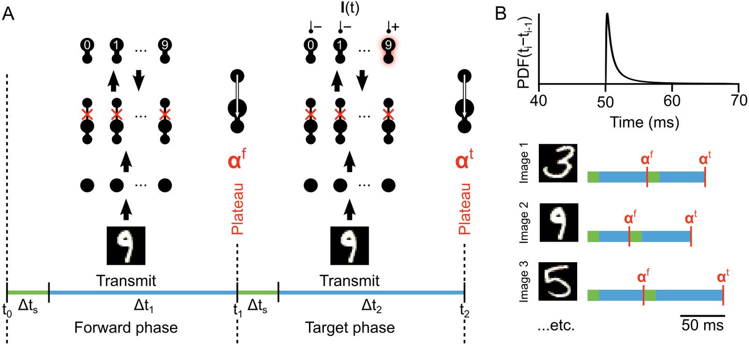
Illustration of network phases for learning.
(A) Illustration of the sequence of network phases that occur for each training example. The network undergoes a forward phase where and a target phase where causes any given neuron to fire at max-rate or be silent, depending on whether it is the correct category of the current input image. In this illustration, an image of a ‘9’ is being presented, so the ’9’ unit at the output layer is activated and the other output neurons are inhibited and silent. At the end of the forward phase the set of plateau potentials are calculated, and at the end of the target phase the set of plateau potentials are calculated. (B) Illustration of phase length sampling. Each phase length is sampled stochastically. In other words, for each training image, the lengths of forward and target phases (shown as blue bar pairs, where bar length represents phase length) are randomly drawn from a shifted inverse Gaussian distribution with a minimum of 50 ms.
Figure 5 with 1 supplement
Co-ordinated errors between the output and hidden layers.
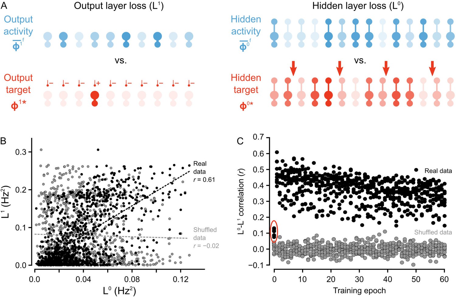
(A) Illustration of output loss function () and local hidden loss function (). For a given test example shown to the network in a forward phase, the output layer loss is defined as the squared norm of the difference between target firing rates and the average firing rate during the forward phases of the output units. Hidden layer loss is defined similarly, except the target is (as defined in the text). (B) Plot of vs. for all of the ‘2’ images after one epoch of training. There is a strong correlation between hidden layer loss and output layer loss (real data, black), as opposed to when output and hidden loss values were randomly paired (shuffled data, gray). (C) Plot of correlation between hidden layer loss and output layer loss across training for each category of images (each dot represents one category). The correlation is significantly higher in the real data than the shuffled data throughout training. Note also that the correlation is much lower on the first epoch of training (red oval), suggesting that the conditions for credit assignment are still developing during the first epoch.
-
Figure 5—source data 1
Fig_5B.csv.
The first two columns of the data file contain the hidden layer loss () and output layer loss () of a one hidden layer network in response to all ‘2’ images in the MNIST test set after one epoch of training. The last two columns contain the same data, except that the data in the third column (Shuffled data ) was generated by randomly shuffling the hidden layer activity vectors. Fig_5C.csv. The first 10 columns of the data file contain the mean Pearson correlation coefficient between the hidden layer loss () and output layer loss () of the one hidden layer network in response to each category of handwritten digits across training. Each row represents one epoch of training. The last 10 columns contain the mean Pearson correlation coefficients between the shuffled hidden layer loss and the output layer loss for each category, across training. Fig_5S1A.csv. This data file contains the maximum eigenvalue of over 60,000 training examples for a one hidden layer network, where and are the mean feedforward and feedback Jacobian matrices for the last 100 training examples.
- https://doi.org/10.7554/eLife.22901.009
Figure 5—figure supplement 1
Weight alignment during first epoch of training.
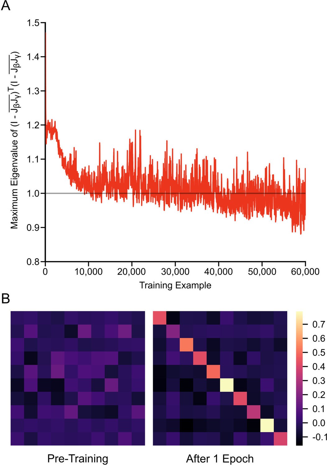
(A) Plot of the maximum eigenvalue of over 60,000 training examples for a one hidden layer network, where and are the mean feedforward and feedback Jacobian matrices for the last 100 training examples. The maximum eigenvalue of drops below one as learning progresses, satisfying the main condition for the learning guarantee described in Theorem one to hold. (B) The product of the mean feedforward and feedback Jacobian matrices, , for a one hidden layer network, before training (left) and after 1 epoch of training (right). As training progresses, the network updates its weights in a way that causes this product to approach the identity matrix, meaning that the two matrices are roughly inverses of each other.
Figure 6 with 1 supplement
Improvement of learning with hidden layers.
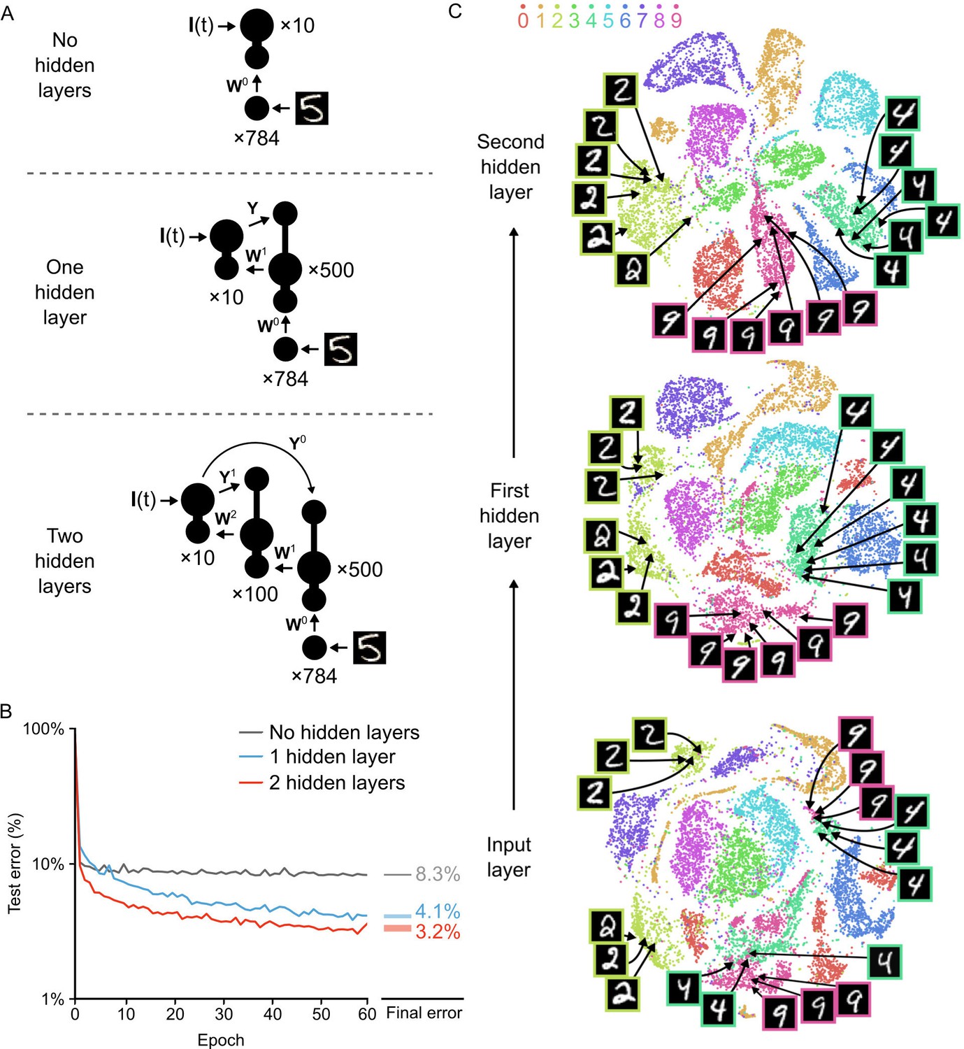
(A) Illustration of the three networks used in the simulations. Top: a shallow network with only an input layer and an output layer. Middle: a network with one hidden layer. Bottom: a network with two hidden layers. Both hidden layers receive feedback from the output layer, but through separate synaptic connections with random weights and . (B) Plot of test error (measured on 10,000 MNIST images not used for training) across 60 epochs of training, for all three networks described in A. The networks with hidden layers exhibit deep learning, because hidden layers decrease the test error. Right: Spreads (min – max) of the results of repeated weight tests () after 60 epochs for each of the networks. Percentages indicate means (two-tailed t-test, 1-layer vs. 2-layer: , ; 1-layer vs. 3-layer: , ; 2-layer vs. 3-layer: , , Bonferroni correction for multiple comparisons). (C) Results of t-SNE dimensionality reduction applied to the activity patterns of the first three layers of a two hidden layer network (after 60 epochs of training). Each data point corresponds to a test image shown to the network. Points are color-coded according to the digit they represent. Moving up through the network, images from identical categories are clustered closer together and separated from images of different categories. Thus the hidden layers learn increasingly abstract representations of digit categories.
-
Figure 6—source data 1
Fig_6B_errors.csv.
This data file contains the test error (measured on 10,000 MNIST images not used for training) across 60 epochs of training, for a network with no hidden layers, a network with one hidden layer, and a network with two hidden layers. Fig_6B_final_errors.csv. This data file contains the results of repeated weight tests () after 60 epochs for each of the three networks described above. Fig_6C.csv. The first column of this data file contains the categories of 10,000 MNIST images presented to a two hidden layer network (after 60 epochs of training). The next three pairs of columns contain the and -coordinates of the t-SNE two-dimensional reduction of the activity patterns of the input layer, the first hidden layer, and the second hidden layer, respectively. Fig_6S1B_errors.csv. This data file contains the test error (measured on 10,000 MNIST images not used for training) across 60 epochs of training, for a one hidden layer network, with synchronized plateau potentials (Regular) and with stochastic plateau potentials. Fig_6S1B_final_errors.csv. This data file contains the results of repeated weight tests () after 60 epochs for each of the two networks described above.
- https://doi.org/10.7554/eLife.22901.012
Figure 6—figure supplement 1
Learning with stochastic plateau times.
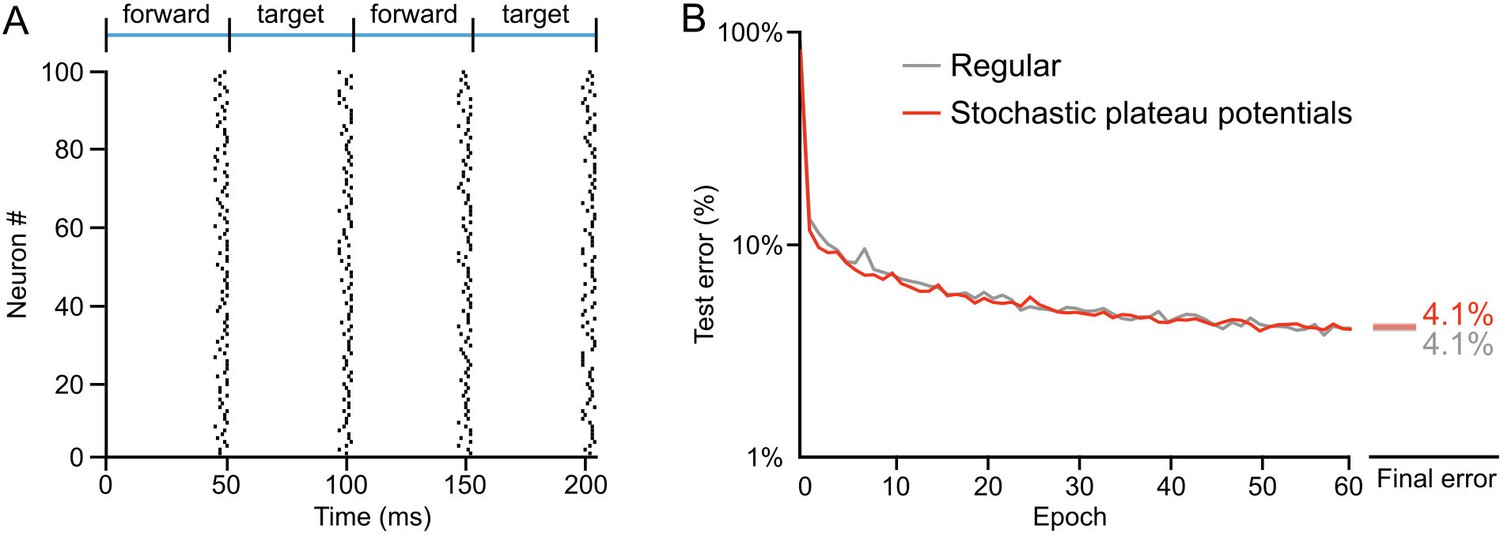
(A) Left: Raster plot showing plateau potential times during presentation of two training examples for 100 neurons in the hidden layer of a network where plateau potential times were randomly sampled for each neuron from a folded normal distribution () that was truncated () such that plateau potentials occurred between 0 ms and 5 ms before the start of the next phase. In this scenario, the apical potential over the last 30 ms was integrated to calculate the plateau potential for each neuron. (B) Plot of test error across 60 epochs of training on MNIST of a one hidden layer network, with synchronized plateau potentials (gray) and with stochastic plateau potentials (red). Allowing neurons to undergo plateau potentials in a stochastic manner did not hinder training performance.
Figure 7
Approximation of backpropagation with local learning rules.
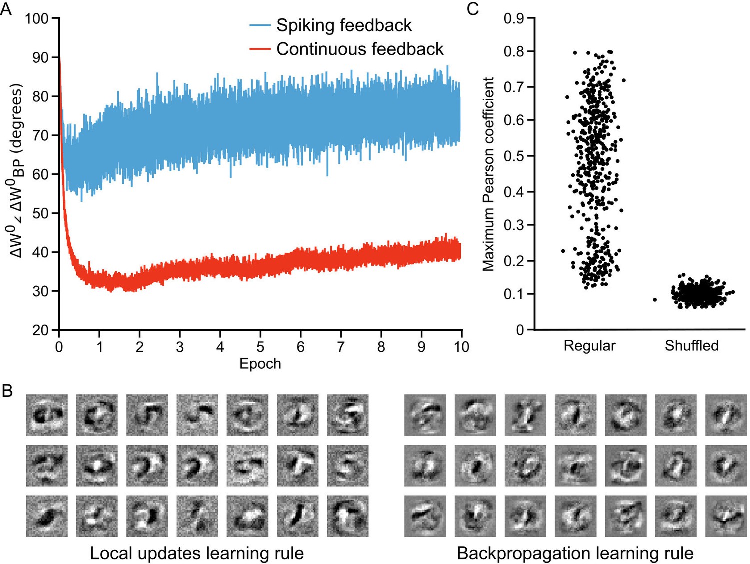
(A) Plot of the angle between weight updates prescribed by our local update learning algorithm compared to those prescribed by backpropagation of error, for a one hidden layer network over 10 epochs of training (each point on the horizontal axis corresponds to one image presentation). Data was time-averaged using a sliding window of 100 image presentations. When training the network using the local update learning algorithm, feedback was sent to the hidden layer either using spiking activity from the output layer units (blue) or by directly sending the spike rates of output units (red). The angle between the local update and backpropagation weight updates remains under during training, indicating that both algorithms point weight updates in a similar direction. (B) Examples of hidden layer receptive fields (synaptic weights) obtained by training the network in A using our local update learning rule (left) and backpropagation of error (right) for 60 epochs. (C) Plot of correlation between local update receptive fields and backpropagation receptive fields. For each of the receptive fields produced by local update, we plot the maximum Pearson correlation coefficient between it and all 500 receptive fields learned using backpropagation (Regular). Overall, the maximum correlation coefficients are greater than those obtained after shuffling all of the values of the local update receptive fields (Shuffled).
-
Figure 7—source data 1
Fig_7A.csv.
This data file contains the time-averaged angle (with a sliding window of 100 images) between weight updates prescribed by our local update learning algorithm compared to those prescribed by backpropagation of error, for a one hidden layer network over 10 epochs of training (600,000 training examples). Fig_7C.csv. The first column of this data file contains the maximum Pearson correlation coefficient between each receptive field learned using our algorithm and all 500 receptive fields learned using backpropagation. The second column of this data file contains the maximum Pearson correlation coefficient between a randomly shuffled version of each receptive field learned using our algorithm and all 500 receptive fields learned using backpropagation.
- https://doi.org/10.7554/eLife.22901.014
Figure 8 with 1 supplement
Conditions on feedback synapses for effective learning.
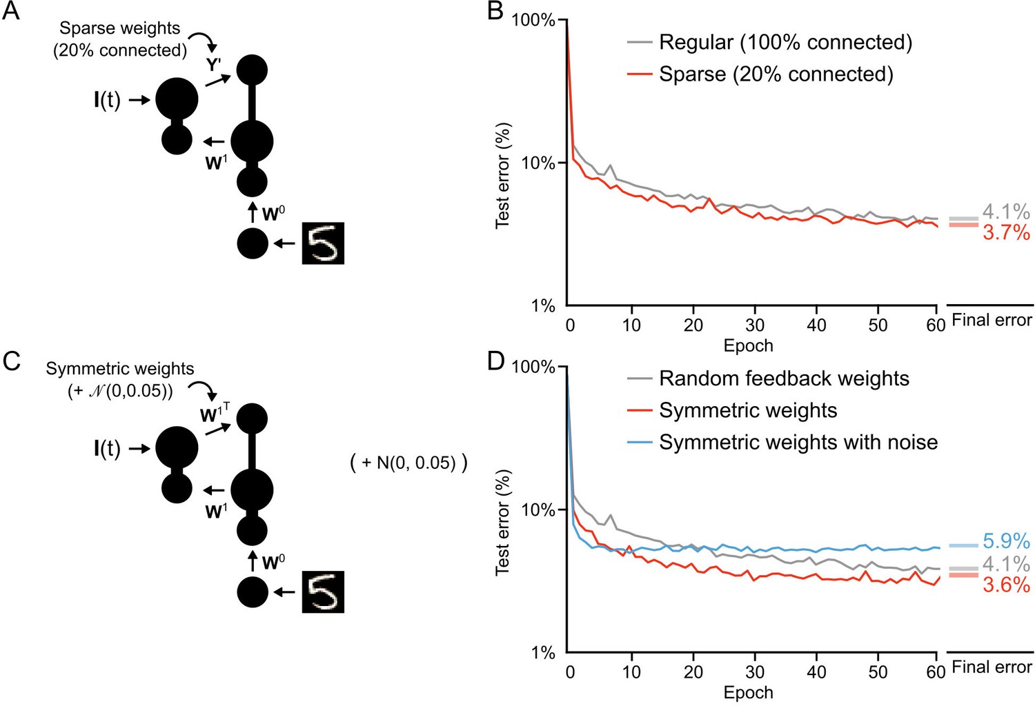
(A) Diagram of a one hidden layer network trained in B, with 80% of feedback weights set to zero. The remaining feedback weights were multiplied by five in order to maintain a similar overall magnitude of feedback signals. (B) Plot of test error across 60 epochs for our standard one hidden layer network (gray) and a network with sparse feedback weights (red). Sparse feedback weights resulted in improved learning performance compared to fully connected feedback weights. Right: Spreads (min – max) of the results of repeated weight tests () after 60 epochs for each of the networks. Percentages indicate mean final test errors for each network (two-tailed t-test, regular vs. sparse: , ). (C) Diagram of a one hidden layer network trained in D, with feedback weights that are symmetric to feedforward weights , and symmetric but with added noise. Noise added to feedback weights is drawn from a normal distribution with variance . (D) Plot of test error across 60 epochs of our standard one hidden layer network (gray), a network with symmetric weights (red), and a network with symmetric weights with added noise (blue). Symmetric weights result in improved learning performance compared to random feedback weights, but adding noise to symmetric weights results in impaired learning. Right: Spreads (min – max) of the results of repeated weight tests () after 60 epochs for each of the networks. Percentages indicate means (two-tailed t-test, random vs. symmetric: , ; random vs. symmetric with noise: , ; symmetric vs. symmetric with noise: , , Bonferroni correction for multiple comparisons).
-
Figure 8—source data 1
Fig_8B_errors.csv.
This data file contains the test error (measured on 10,000 MNIST images not used for training) across 60 epochs of training, for our standard one hidden layer network (Regular) and a network with sparse feedback weights. Fig_8B_final_errors.csv. This data file contains the results of repeated weight tests () after 60 epochs for each of the two networks described above. Fig_8D_errors.csv. This data file contains the test error (measured on 10,000 MNIST images not used for training) across 60 epochs of training, for our standard one hidden layer network (Regular), a network with symmetric weights, and a network with symmetric weights with added noise. Fig_8D_final_errors.csv. This data file contains the results of repeated weight tests () after 60 epochs for each of the three networks described above. Fig_8S1_errors.csv. This data file contains the test error (measured on 10,000 MNIST images not used for training) across 20 epochs of training, for a one hidden layer network with regular feedback weights, sparse feedback weights that were amplified, and sparse feedback weights that were not amplified. Fig_8S1_final_errors.csv. This data file contains the results of repeated weight tests () after 20 epochs for each of the three networks described above.
- https://doi.org/10.7554/eLife.22901.017
Figure 8—figure supplement 1
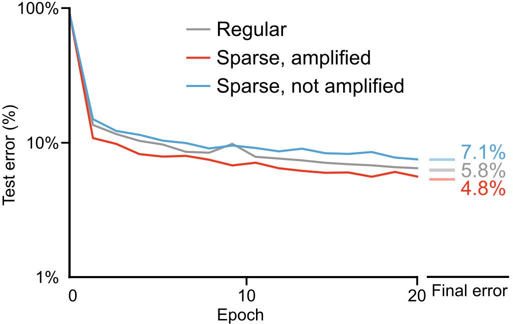
Importance of weight magnitudes for learning with sparse weights.
Plot of test error across 20 epochs of training on MNIST of a one hidden layer network, with regular feedback weights (gray), sparse feedback weights that were amplified (red), and sparse feedback weights that were not amplified (blue). The network with amplified sparse feedback weights is the same as in Figure 8A and B, where feedback weights were multiplied by a factor of 5. While sparse feedback weights that were amplified led to improved training performance, sparse weights without amplification impaired the network’s learning ability. Right: Spreads (min – max) of the results of repeated weight tests () after 20 epochs for each of the networks. Percentages indicate means (two-tailed t-test, regular vs. sparse, amplified: , ; regular vs. sparse, not amplified: , ; sparse, amplified vs. sparse, not amplified: , , Bonferroni correction for multiple comparisons).
Figure 9
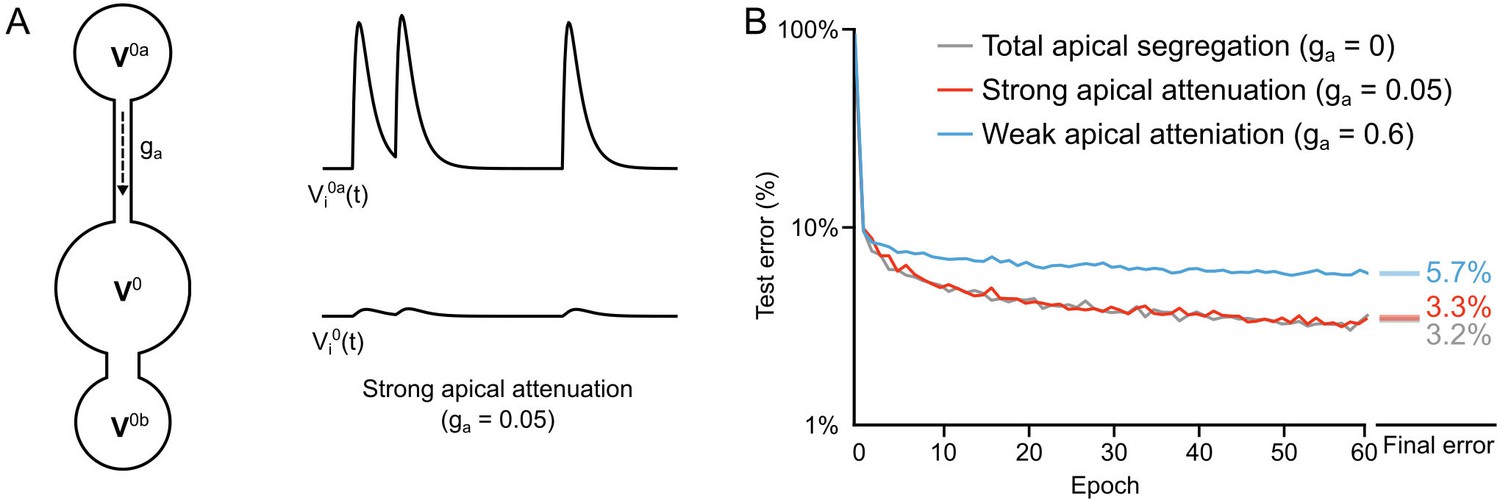
Importance of dendritic segregation for deep learning.
(A) Left: Diagram of a hidden layer neuron. represents the strength of the coupling between the apical dendrite and soma. Right: Example traces of the apical voltage in a single neuron and the somatic voltage in response to spikes arriving at apical synapses. Here , so the apical activity is strongly attenuated at the soma. (B) Plot of test error across 60 epochs of training on MNIST of a two hidden layer network, with total apical segregation (gray), strong apical attenuation (red) and weak apical attenuation (blue). Apical input to the soma did not prevent learning if it was strongly attenuated, but weak apical attenuation impaired deep learning. Right: Spreads (min – max) of the results of repeated weight tests () after 60 epochs for each of the networks. Percentages indicate means (two-tailed t-test, total segregation vs. strong attenuation: , ; total segregation vs. weak attenuation: , ; strong attenuation vs. weak attenuation: , , Bonferroni correction for multiple comparisons).
-
Figure 9—source data 1
Fig_9B_errors.csv.
This data file contains the test error (measured on 10,000 MNIST images not used for training) across 60 epochs of training, for a two hidden layer network, with total apical segregation (Regular), strong apical attenuation and weak apical attenuation. Fig_9B_final_errors.csv. This data file contains the results of repeated weight tests () after 60 epochs for each of the three networks described above.
- https://doi.org/10.7554/eLife.22901.019
Figure 10

An experiment to test the central prediction of the model.
(A) Illustration of the basic experimental set-up required to test the predictions (generic or specific) of the deep learning with segregated dendrites model. To test the predictions of the model, patch clamp recordings could be performed in neocortical pyramidal neurons (e.g. layer 5 neurons, shown in black), while the top-down inputs to the apical dendrites and bottom-up inputs to the basal dendrites are controlled separately. This could be accomplished optically, for example by infecting layer 4 cells with channelrhodopsin (blue cell), and a higher-order cortical region with a red-shifted opsin (red axon projections), such that the two inputs could be controlled by different colors of light. (B) Illustration of the specific experimental prediction of the model. With separate control of top-down and bottom-up inputs a synaptic plasticity experiment could be conducted to test the central prediction of the model, that is that the timing of apical inputs relative to basal inputs should determine the sign of plasticity at basal dendrites. After recording baseline postsynaptic responses (black lines) to the basal inputs (blue lines) a plasticity induction protocol could either have the apical inputs (red lines) arrive early during basal inputs (left) or late during basal inputs (right). The prediction of our model would be that the former would induce LTD in the basal synapses, while the later would induce LTP.
Tables
Table 1
List of parameter values used in our simulations.
https://doi.org/10.7554/eLife.22901.021| Parameter | Units | Value | Description |
|---|---|---|---|
| ms | 1 | Time step resolution | |
| Hz | 200 | Maximum spike rate | |
| ms | 3 | Short synaptic time constant | |
| ms | 10 | Long synaptic time constant | |
| ms | 30 | Settle duration for calculation of average voltages | |
| S | 0.6 | Hidden layer conductance from basal dendrites to the soma | |
| S | 0, 0.05, 0.6 | Hidden layer conductance from apical dendrites to the soma | |
| S | 0.6 | Output layer conductance from dendrites to the soma | |
| S | 0.1 | Leak conductance | |
| mV | Resting membrane potential | ||
| F | Membrane capacitance | ||
| – | Hidden layer error signal scaling factor | ||
| – | Output layer error signal scaling factor |
Additional files
-
Transparent reporting form
- https://doi.org/10.7554/eLife.22901.022
Download links
A two-part list of links to download the article, or parts of the article, in various formats.
Downloads (link to download the article as PDF)
Open citations (links to open the citations from this article in various online reference manager services)
Cite this article (links to download the citations from this article in formats compatible with various reference manager tools)
Towards deep learning with segregated dendrites
eLife 6:e22901.
https://doi.org/10.7554/eLife.22901


