Single-protein detection in crowded molecular environments in cryo-EM images
- Howard Hughes Medical Institute, United States
- Max Planck Institute of Neurobiology, Germany
Figures
Figure 1 with 2 supplements
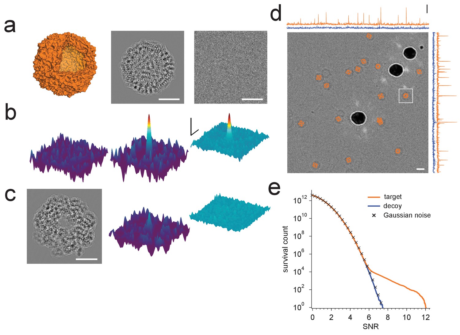
Protein detection in vitreous ice.
(a) From the left: apoferritin structure, template at 220 nm underfocus, image of a single apoferritin in ice at 220 nm underfocus with 1200 electrons/nm2. (b) Cross-correlograms (CCGs), left to right: template five degrees rotated around z-axis from best orientation, template at best orientation, maximum intensity projection (MIP) across all template orientations. (c) GroEL (decoy) template at 220 nm underfocus, single CCG, and MIP. (d) Image at 2200 nm underfocus. Orange octahedrons indicate the orientation and location of CCG peak values from a full search of an image of the same area at 220 nm underfocus taken before the displayed image. Traces along right and top edge: horizontal and vertical projections of the maximum across orientations (orange: apoferritin, blue: GroEL; blue traces offset by 1.5 SNR units for clarity). Note the dark rings, which presumably correspond to apoferritin particles (the large round objects are gold particles). The boxed region indicates the image region used for (a), (b), and (c). (e) CCG value survival histograms (number of CCG values above a given SNR) for apoferritin (orange), GroEL (blue), and as expected for Gaussian noise (crosses). Scale bars are 5 nm for images and 1 nm for surface plots in (a)-(c), 5 SNR units for surface plots in (b), and 10 nm and 3 SNR units in (d). The top and bottom ends of the amplitude scale bar in (d) correspond to SNRs of 10 and 13, respectively.
Figure 1—figure supplement 1
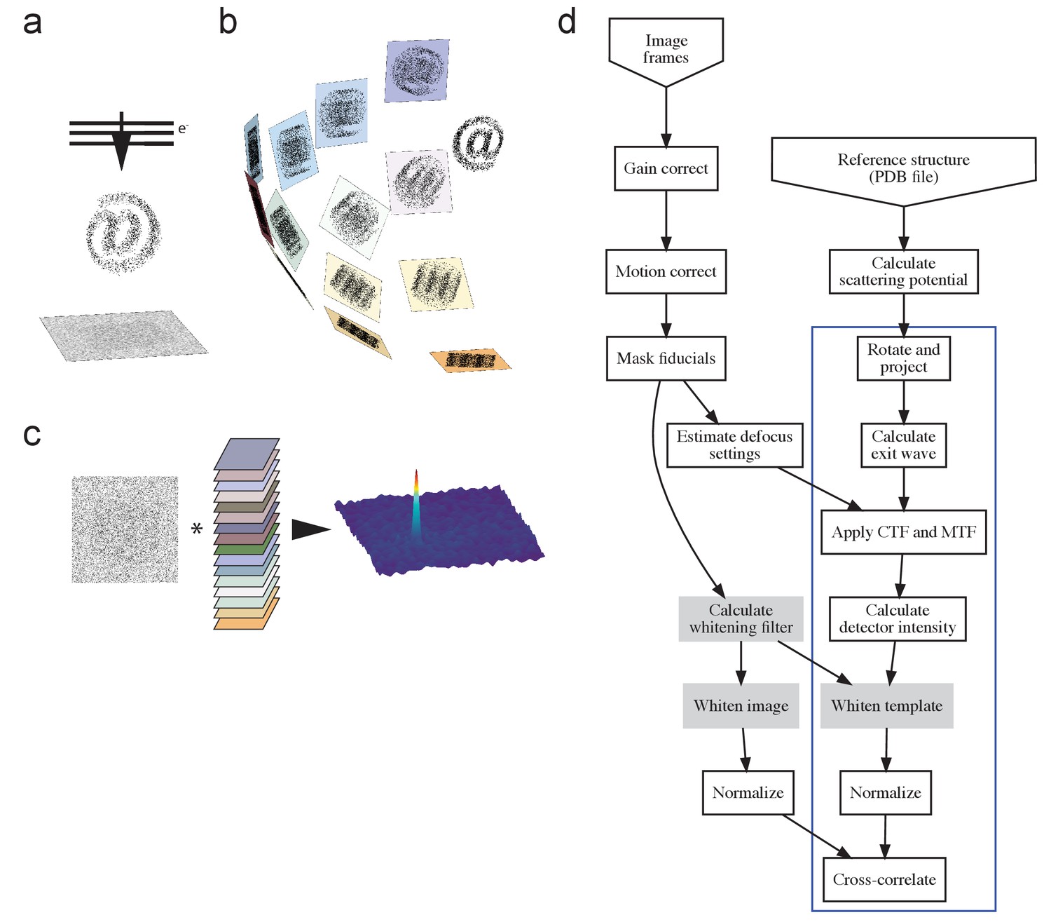
The process.
(a) TEM acquisition, with @ representing the target protein, (b) generation of the template set, and c) matching. (d) Flow-chart illustrating the process. Blue box indicates steps repeated for each template orientation, with filtering steps (used where described in the main text) shaded gray. PDB, Protein Data Bank; CTF, contrast transfer function; MTF, modulation transfer function.
Figure 1—figure supplement 2
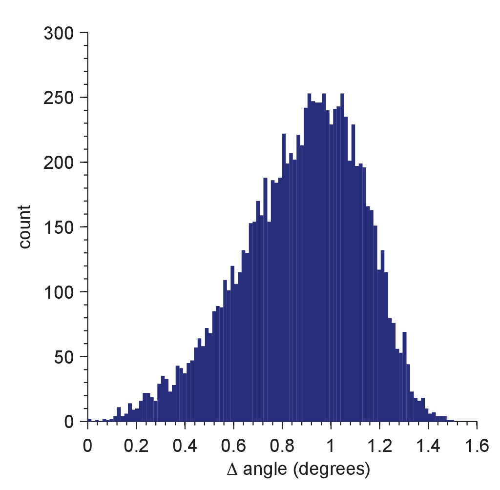
Distribution of residual orientation mismatches for a test set of 10,000 random orientations.
The mismatch for a member of the test set is the minimum of the angular differences between the tested orientation and all members of the Hopf set used for full searches (2,359,296 orientations; simple grid, resolution = 5; Yershova, A., Jain, S., LaValle, S.M. and Mitchell, J.C., Int. J. Rob. Res 29(7):801–812, 2010). The test-set orientations were generated using the randRot method in the quaternion classdef (M. Tincknell, https://www.mathworks.com/matlabcentral/fileexchange/33341-quaternion-m, 21 July 2016).
Figure 2 with 2 supplements
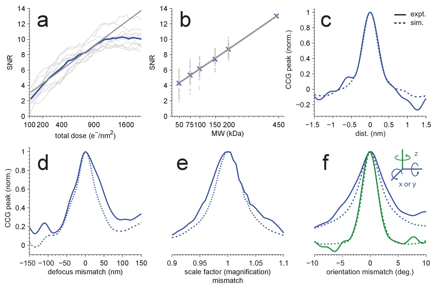
Detection sensitivity.
(a,b) CCG values at the correct location and orientation vs. electron exposure for the particle’s full structure (a), and vs. the MW (b) for partial structures. The ten (panel a) or two (panel b) particles with the largest SNRs in Figure 1(d) were used. Individual and averaged values are shown in gray and blue, respectively. Gray lines show fits to the averages (see Results). (c–f) Peak correlogram values vs. lateral position, focus mismatch, scale factor (magnification) mismatch, and orientation mismatch, all normalized to the maximum. Dashed lines are from simulations, solid lines from experiments. Traces in (c–f) are averages of two particles.
Figure 2—figure supplement 1
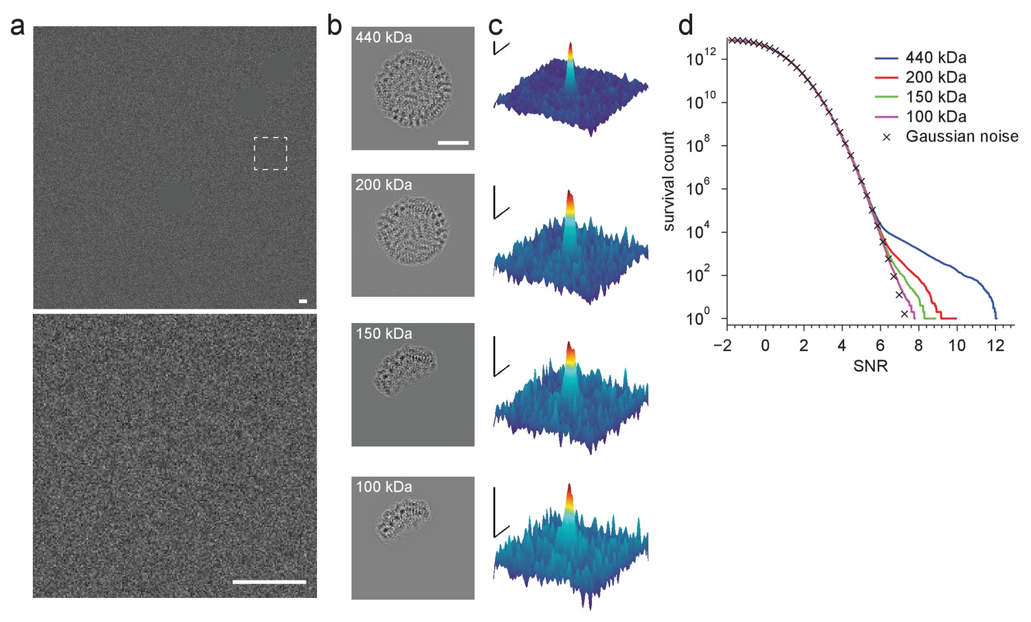
Detection using template fragments.
(a) Experimental image taken at 220 nm underfocus. Shown are the full field-of-view (upper) and a region centered around a particle (lower, boxed region in upper, contrast and offset adjusted). Gold fiducial particles in the image are masked (Materials and methods). (b) Example templates for fragments of the full apoferritin structure ranging in size (indicated in each panel) from 100 to 440 kDa. (c) Full-search CCG MIPs centered on a particle (boxed region in a). (d) CCG value survival histograms (number of CCG values above a given SNR) from full searches for the indicated fragment structures. Scale bars are 5 nm in (a) and (b), and 1 nm and 2 SNR units in (c).
Figure 2—figure supplement 2
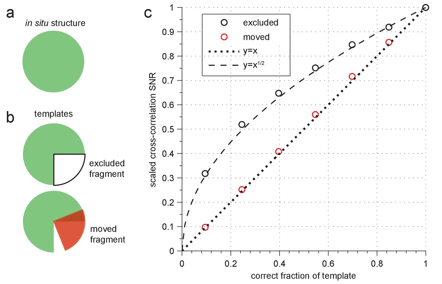
Sensitivity to template errors.
(a–b) Schematic diagram of two template-mismatch cases. (a) An in situ structure and (b) structures used to generate templates for cross-correlation against the in situ structure. (c) SNR (scaled relative to maximum) from cross-correlating a simulated image of apoferritin based on a known structure (PDB: 2W0O) against templates based on the same structure, but now with fragments either excluded (black circles) or moved to an incorrect location (red circles). Dashed and dotted lines show the indicated polynomial curves for reference.
Figure 3 with 1 supplement

Detection against background.
(a) Simulated images of a single apoferritin in ice without (left) and with (right) a dense protein background (BSA at 37.5 kDa-nm−2), at 70 nm and 2000 nm underfocus as well as for a perfect phase-plate microscope (PPM). To the right of each image the corresponding maximum-projected CCG from a full orientation search is shown. (b) Squared contrast transfer functions (CTFs) for 70 nm (green) and 2000 nm (red) underfocus, and squared whitening filters for 70 nm underfocus (black) and the PPM (purple). (c) Power spectral densities for the apoferritin template alone (light blue) and for simulated images of the protein background alone using the PPM (black), at 70 nm underfocus (green), and at 2000 nm underfocus (red). Spatial scale bars are 10 nm for the images and 2 nm for CCGs. SNR bars are 5 and 2 SNR units for left and right columns in (a) respectively.
Figure 3—figure supplement 1
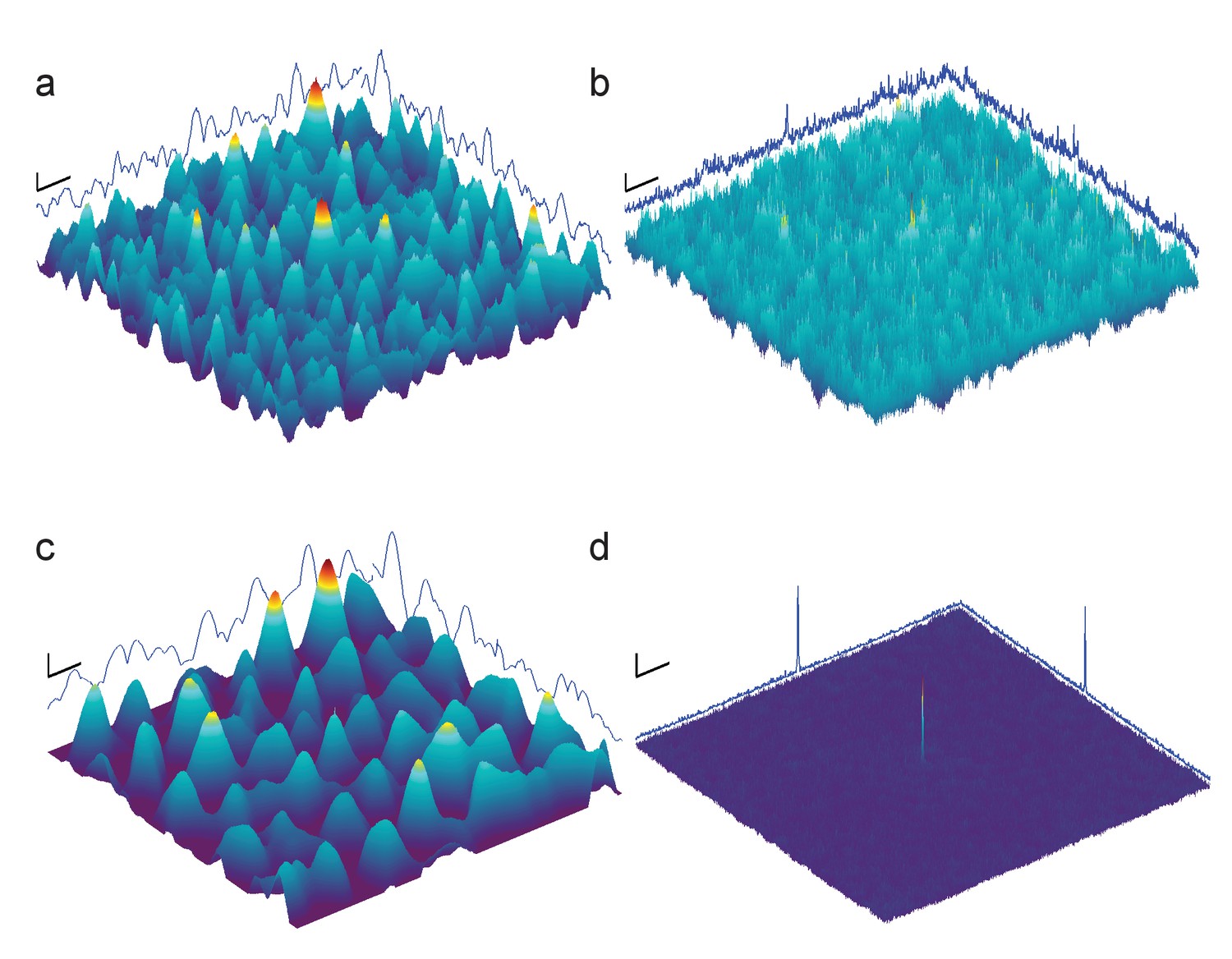
Full-search CCG MIPs for simulated images of apoferritin with BSA background, 2000 nm underfocus (Figure 3a, right column), without (a) and with (b) pre-whitening.
Traces along edges: one-dimensional maximum intensity projections of the CCG MIPs. (c–d) Same as (a–b) but using simulations assuming a perfect phase-plate microscope (PPM). Scale bars are 5 nm in (a–d), 1 SNR unit in (a–c), and 4 SNR units in (d).
Figure 4

Optimized detection.
(a) Whitened templates and simulated images together with the corresponding maximum-projected CCGs for apoferritin with a BSA background of 37.5 kDa/nm2 (same as in Figure 3a right except for whitening). (b) SNR vs. defocus for simulated images of apoferritin, all with 50 nm of ice but only some with BSA background (black, green, orange), with whitening (green, orange), with randomly scattered carbon atoms (18.7 kDa-nm−2) as background (gray), and with perfect illumination coherence (orange). Scale bars are 10 nm for images and 2 nm and 2 SNR units for CCGs.
Figure 5 with 1 supplement
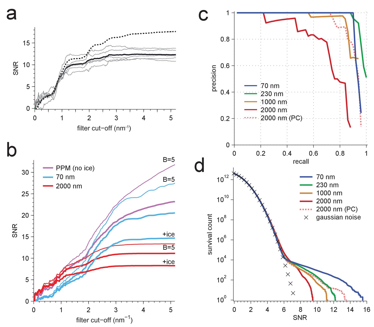
Resolution dependence and performance.
(a,b) SNR vs. low pass-filter cut-off; (a) for five of the particles in Figure 1d (individual trace: thin gray, average: thick black) and the average of two simulations (dashed) using the same optical parameters as for two of the experimental particles; (b) for simulated images using the protein background, whitening and B-factors as in the PDB file (thick traces) or B = 5 Å2 (thin traces) and ice or no ice as indicated. (c) Simulated-image precision-recall curves for 50 randomly oriented and positioned apoferritin molecules with 37.5 kDa-nm−2 of BSA background at underfocus values as indicated. Full orientation searches with whitening and standard imaging parameters were used, except in one case, which used perfect illumination coherence (2000 nm, PC). (d) CCG value survival histograms (number of CCG values above a given SNR) from full searches of simulated images with parameters as indicated. Crosses: Gaussian noise (same as Figure 1e).
Figure 5—figure supplement 1
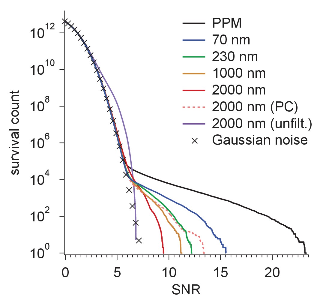
Survival histograms for various simulated image and template-matched conditions as in Figure 5d, additionally showing results for a PPM and a 2000 nm underfocus image that was not whitened (all other traces reflect whitening).
PPM, phase-plate microscope; PC, perfect coherence.
Figure 6
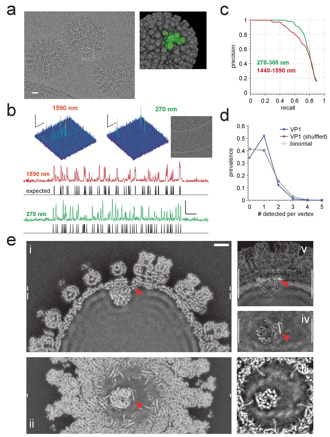
Application to rotavirus.
(a) Left: rotavirus DLPs imaged at 1590 nm underfocus with 1600 electrons nm−2. Right: surface-rendered electron density of the DLP with one ASU highlighted in green. (b) MIP CCGs from searches for the ASU in images taken at 1590 nm and 270 nm underfocus, respectively. Top: regions around an ASU peak and (only for 270 nm) the corresponding image region with inner and outer capsid edges indicated by dashed lines. The corresponding region in the 1590 nm image is indicated by the dashed square in a). Below: maximum projections over all orientations and one spatial direction and the expected peak locations (black traces). (c) Precision-recall curves for detection of the ASU; five DLPs each acquired with an underfocus between 1440 and 1590 nm (red) and between 270 and 300 nm (green). (d) Prevalence of the number of VP1 polymerase proteins per fivefold vertex detected in a constrained search (dark blue) and after randomly permuting vertex labels (gray, crosses) and for a binomial distribution with the same mean detection rate (dashed, circles). (e) Density map from a VP1 detection-triggered reconstruction of a rotavirus DLP: i) MIP of a 1 nm thick subset (extent indicated by white vertical bars in (ii). Note the polymerase to the left of the RNA exit channel in the capsid. ii) Orthogonal MIP of a different subset (location indicated by white vertical bars in (i). iii) average over a 0.5 nm thick subset (location indicated by gaps in white vertical bars in (i). Note the presumptive RNA helix wrapped around the polymerase. iv) and v) MIPs of the difference between reconstructed and a simulated potential based on PDB:4F5X (projected ranges given by white vertical lines in (v) and (iv), respectively). Red arrow indicates possible VP3 helix. Scale bars are 10 nm in (a), 5 nm and 3 SNR units in (b) and 5 nm in (e).
Additional files
-
Supplementary file 1
3D reconstruction.
Stack of sections from a reconstruction of the rotavirus RNA polymerase VP1 bound near a fivefold vertex in a double-layered particle (DLP; odd frames), interleaved with sections through a simulated DLP based on the model used for VP1 template generation (even frames). Voxel size is 0.1023 nm.
- https://doi.org/10.7554/eLife.25648.014
-
Supplementary file 2
Sample input files for TEM-simulator v.1.3 (Rullgard et al., J. Microscopy 243(3):234–256, 2011) to calculate expected intensity distributions at the detector, and expected output files.
Images generated by TEM-simulator and used here were downsampled twofold, to a pixel size of 0.0965 nm, by Fourier cropping before substituting each pixel intensity with a new value drawn from a Poisson distribution with the same mean. Further details of the included files are provided in README.txt in the. zip folder.
- https://doi.org/10.7554/eLife.25648.015
-
Supplementary file 3
CCG values from the constrained VP1 search.
Indices for the five-dimensional matrix (2 × 3296 × 12 × 5 × 5) correspond to: target or control template (1 or 2); DLP image number (1–3296); vertex number (1–12); position within the vertex (1–5); pixel neighborhood (1–5), with #3 the center pixel and 1, 2, 4, and 5 the adjacent pixels.
- https://doi.org/10.7554/eLife.25648.016
-
Supplementary file 4
Results from full searches described in the main text (see Supplementary file 5 for file names and descriptions).
Each file contains a matrix of the 100,000 highest CCG values in descending order (column 1) and the corresponding LOCs (columns 2–7). Locations in the image (columns 2 and 3, in nm) are given as x and y distances from one corner pixel. Template orientations (columns 4–7) are given as the four sequential elements of a unit quaternion vector q. An equivalent rotation matrix, R, may be calculated from this representation as:
- https://doi.org/10.7554/eLife.25648.017
-
Supplementary file 5
List of files included in Supplementary file 4.
Columns Δf1, Δf2, and αast provide defocus parameters (Rohou and Grigorieff, 2015) assumed in template generation.
- https://doi.org/10.7554/eLife.25648.018
Download links
A two-part list of links to download the article, or parts of the article, in various formats.
Downloads (link to download the article as PDF)
Open citations (links to open the citations from this article in various online reference manager services)
Cite this article (links to download the citations from this article in formats compatible with various reference manager tools)
Single-protein detection in crowded molecular environments in cryo-EM images
eLife 6:e25648.
https://doi.org/10.7554/eLife.25648


