Microsaccadic sampling of moving image information provides Drosophila hyperacute vision
- Beijing Normal University, China
- University of Sheffield, United Kingdom
- Champalimaud Center for the Unknown, Portugal
- Cambridge University, United Kingdom
Figures
Figure 1 with 1 supplement

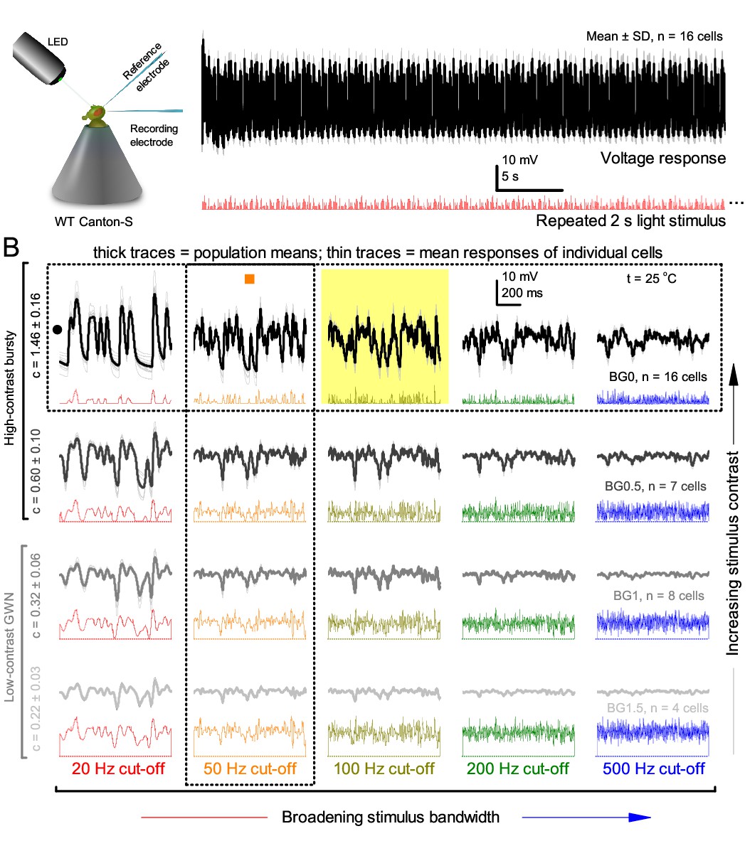
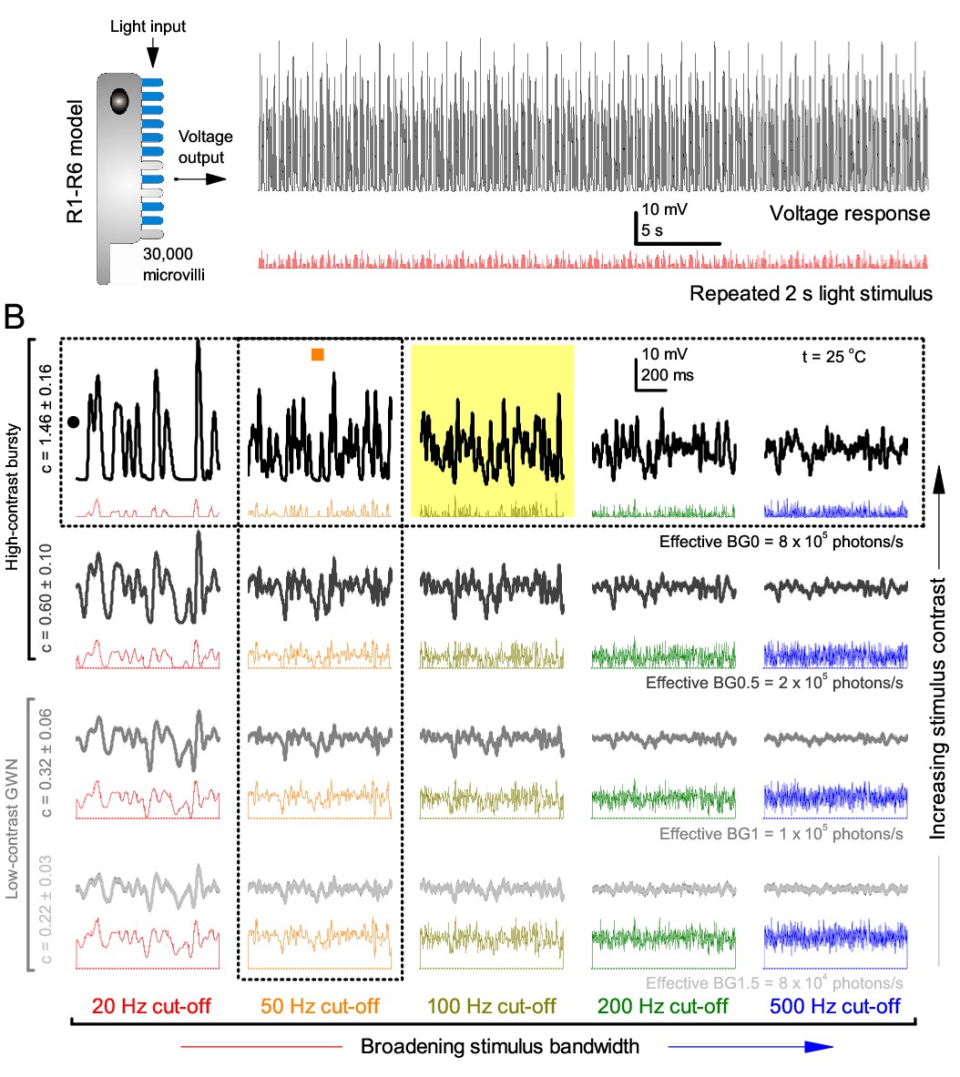
Photoreceptors respond best to high-contrast bursts.
(A) Schematic of intracellular recordings to repeated bursty light intensity time series (20 Hz bandwidth). Responses changed little (minimal adaptation) during bursts. (B) Testing a R1-R6 photoreceptor’s diurnal encoding gamut. Means (thick traces) and 20 individual responses (thin; near-perfectly overlapped) to 20 different stimuli; each with a specific bandwidth (columns: from 20 Hz, red, to 500 Hz, blue) and mean contrast (rows). Reducing the background (BG) of Gaussian white-noise stimuli (GWN; 2-unit peak-to-peak modulation) from bright (1.5-unit, bottom) to dark (0-unit, top) halved their modulation, generating bursts of increasing contrast: the lower the BG, the higher the contrast. Left-top: responses from (A). Yellow box: maximum information responses. Arrows: dark intervals. Because of half-Gaussian waveforms, light bursts carried fewer photons (see Figure 2—figure supplement 3). Yet their larger responses comply with the stochastic adaptive visual information sampling theory (Song et al., 2012; Song and Juusola, 2014; Juusola et al., 2015) (Appendixes 1–3), whereby dark intervals rescue refractory microvilli for transducing high-frequency (1–20 ms) saccadic photon surges (of high contrast) into quantum bumps efficiently. Thus, larger responses would incorporate more bumps. Recordings are from the same photoreceptor. Vertical dotted rectangle (orange square) and horizontal rectangle (black circle): responses for contrast and bandwidth analyses in Figure 2A. Similar R1-R6 population data is in Figure 1—figure supplement 1.
-
Figure 1—source data 1
Intracellular voltage responses of the same R1-R6 photoreceptor to very bright 20 Hz, 50 Hz, 100 Hz, 200 Hz and 500 Hz bursty light stimuli at BG0 (darkness).
- https://doi.org/10.7554/eLife.26117.005
-
Figure 1—source data 2
Intracellular voltage responses of the same R1-R6 photoreceptor to very bright 20 Hz, 50 Hz, 100 Hz, 200 Hz and 500 Hz bursty light stimuli at BG0.5.
- https://doi.org/10.7554/eLife.26117.006
-
Figure 1—source data 3
Intracellular voltage responses of the same R1-R6 photoreceptor to very bright 20 Hz, 50 Hz, 100 Hz, 200 Hz and 500 Hz bursty light stimuli at BG1.
- https://doi.org/10.7554/eLife.26117.007
-
Figure 1—source data 4
Intracellular voltage responses of the same R1-R6 photoreceptor to very bright 20 Hz, 50 Hz, 100 Hz, 200 Hz and 500 Hz bursty light stimuli at BG1.5.
- https://doi.org/10.7554/eLife.26117.008
Figure 1—figure supplement 1
R1-R6 output varies more cell-to-cell than trial-to-trial (cf.Figure 1) but show consistent stimulus-dependent dynamics over the whole encoding range.
(A) The mean voltage response and SD of 15 R1-R6 cells to the same repeated 20 Hz bandwidth bursts. Photoreceptor output adapts within ~2 s to the stimulation. (B) Population means (thick) and 4–16 mean voltage responses of individual photoreceptors (thin traces) to 20 different stimuli; each with specific bandwidth (columns: from 20 Hz, red to 500 Hz, blue) and mean contrast (rows). Stimulation changes from Gaussian white-noise (GWN; bottom) to bursts (top) with the light background: from BG0 (dark) to BG1.5 (very bright). Left top: the traces from (A). The yellow box indicates the responses with the highest entropy and information content. Vertical dotted rectangle (orange square) and horizontal rectangle (black circle): responses for contrast and bandwidth analyses in Figure 2—figure supplement 1A. All recordings were done at 25°C. Compare this data to Figure 1.
Figure 2 with 4 supplements

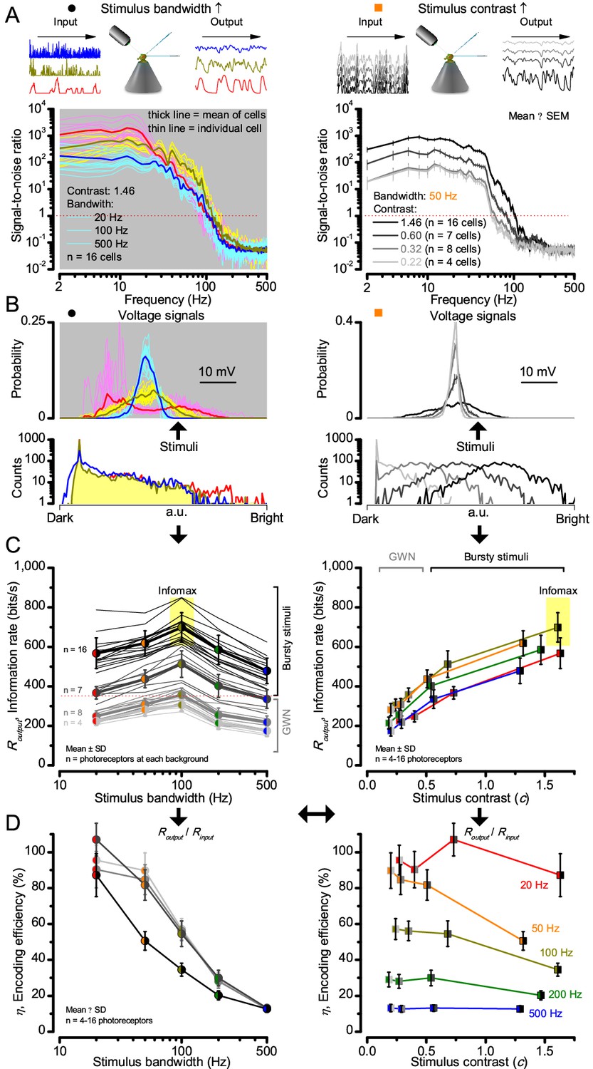
High-contrast bursts drive maximal encoding.
A R1-R6’s information transfer to high-frequency 100 Hz bursts exceeded 2-to-4-times the previous estimates. (A) Response signal-to-noise ratio (SNR, left) to 20 (red), 100 (yellow) and 500 Hz (blue) bursts, and to 50 Hz bandwidth stimuli of different contrasts (right); data from Figure 1. SNR increased with contrast (right), reaching the maximum (~6,000) for 20 Hz bursts (left, red) and the broadest frequency range for 100 Hz bursts (yellow). (B) Skewed bursts drove largely Gaussian responses (exception: 20 Hz bursts, red), with 100 Hz bursts evoking the broadest amplitude range (yellow). (C) Information transfer peaked for 100 Hz stimuli, irrespective of contrast (or BG; left), having the global maximum of ~850 bits/s (capacity, infomax) for the high-frequency high-contrast bursts. (D) Encoding efficiency, the ratio between input and output information (Routput/Rinput), was > 100% for 20 Hz bursts. Extra information came from the neighboring cells. Rinput at each BG was determined for the optimal mean light intensity, which maximized a biophysically realistic photoreceptor model’s information transfer (Appendix 2). Encoding efficiency fell with stimulus bandwidth but remained more constant with contrast. Population dynamics are in Figure 2—figure supplement 1.
Figure 2—figure supplement 1
Signaling performance vary cell-to-cell but adapts similarly to given stimulus statistics.
(A) Response signal-to-noise ratios (SNR) to 20 (red), 100 (yellow) and 500 Hz (blue) bandwidth (left) saccadic bursts, and to 50 Hz bandwidth stimuli of different contrasts (right); color scheme as in Figure 1. SNR increases with contrast (right), reaching (in some cells)~6000 maximum for 20 Hz bursts (left, red). All R1-R6s showed the broadest frequency range for 100 Hz bursts (yellow). (B) Highly skewed bursts drove mostly Gaussian responses (exception: 20 Hz, red), with 100 Hz bursts evoking the broadest amplitude range (yellow). (C) Information transfer of all cells peaked for 100 Hz stimuli, irrespective of the tested contrast (or BG; left), having global maxima (infomax) between 600–850 bits/s (yellow box). (D) Mean encoding efficiency (Routput/Rinput) reached >100% for 20 Hz bursts, with its extra information coming from the neighboring cells. For determining Rinput see Figure 3. Encoding efficiency fell with increasing stimulus bandwidth, but less with contrast. Note: encoding efficiency for bursts (ηburst; black trace, left) was lower than for GWNs (ηGWN; grey and light grey traces). Because photomechanical adaptations let optimally 8-times brighter intensity modulation (photon absorption rate) through for high-contrast bursts (8 × 10⁵ photons/s) than for GWN (1 × 10⁵ photons/s), their input information is higher; . Thus, whilst , (Appendix 2).
Figure 2—figure supplement 2
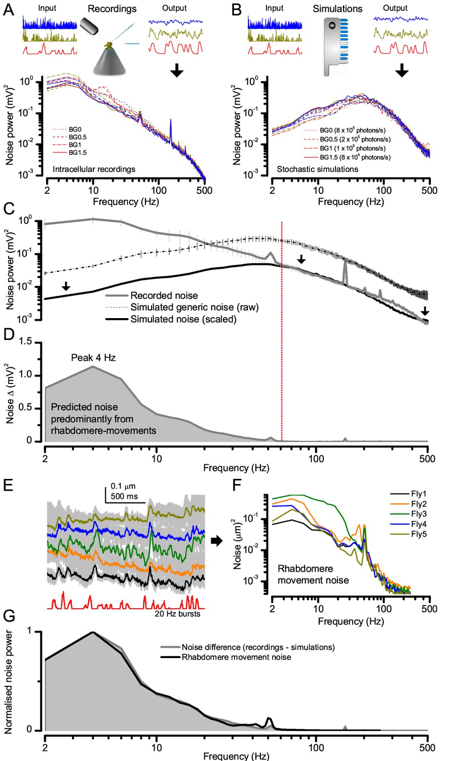
Light-adapted R1-R6 noise is similar for all the test stimuli, with its high-frequencies reflecting the mean quantum bump shape and its low-frequencies the rhabdomere jitter.
(A) Photoreceptor noise (from Figure 1) remained largely constant for all the test stimuli; extracted from the responses (output) to stimulus repetition (input); see Materials and methods. (B) Corresponding photoreceptor noise of the model (Song et al., 2012; Song and Juusola, 2014) simulations was also broadly constant but lacked the recordings’ low-frequency noise in (A). (C) The mean simulated noise power ascends with membrane impedance, which here was larger than that in the recordings in (A). Yet, the high-frequency parts of the real and simulated noise (>60 Hz), indicating the corresponding average light-adapted quantum bump waveform (Wong et al., 1982; Juusola and Hardie, 2001b; Juusola and Hardie, 2001a; Song et al., 2012; Song and Juusola, 2014), sloped similarly. (D) Overlaying these exposed the low-frequency noise difference (<60 Hz). Our results (Figure 8) predicted that this difference was a by-product of photomechanical rhabdomere and eye muscle movements, which the simulations lacked. (E) Mean rhabdomere movement responses (± SD, grey) in five different flies to the same repeated 20 Hz high-contrast bursts. These were smaller than those to 1 s flashing (Figure 8E, Appendix 7). (F) Average variability of the recording series (mean – individual response) shown as rhabdomere movement noise power spectra. (G) Mean rhabdomere movement noise (black trace; from F) matched its prediction (grey; from D). Therefore, the recordings’ extra noise resulted from variable rhabdomere contractions; jittering light input to R1-R6s. Crucially, this noise is minute; for 20 Hz saccadic bursts,~1/6,000 of R1-R6 signal power (Figure 2A).
Figure 2—figure supplement 3
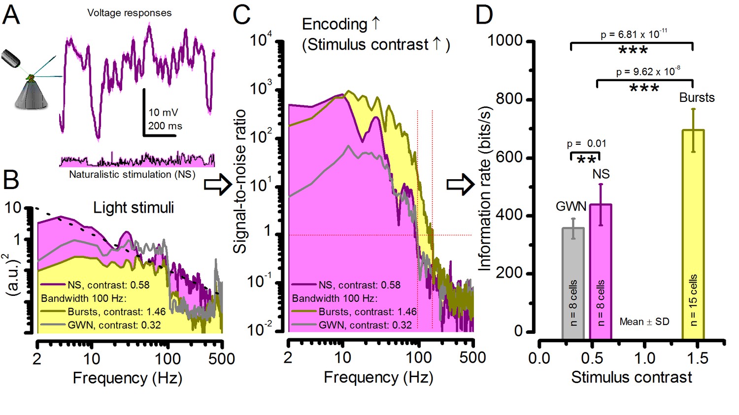
Strong responses to naturalistic stimulation (NS) carry only about half the information of the strongest responses to bursts.
(A) The mean (signal; purple) and voltage responses (pink) of a R1-R6 photoreceptor to naturalistic light intensity time series. (B) At the light source, NS (purple), which is dominated by low-frequency transitions between darker and brighter events, had higher power than GWN (grey) or bursty high-contrast stimuli (yellow), but its mean contrast (0.58) is between the other two. (C) Signal-to-noise ratio of responses to NS has a similar low-frequency maximum to responses to bursty 100 Hz stimuli, but lower values at high-frequencies, similar to GWN-driven responses (grey). Both of these signaling performance estimates are from the same R1-R6 in (A). (D) Information transfer rate in photoreceptor output directly depends upon the mean stimulus contrast. Photoreceptors encode more information during naturalistic stimulation than during GWN stimulation (see also: Song and Juusola, 2014). But encoding can further double during high-contrast bursts, which utilize better the refractory sampling dynamics of 30,000 microvilli, generating the largest sampling rate changes. Significance by two-tailed t-test. For more explanation, see Appendix 3.
Figure 2—figure supplement 4
Drosophila R1-R6 photoreceptor output information transfer rate estimates to bursty stimuli are consistent.
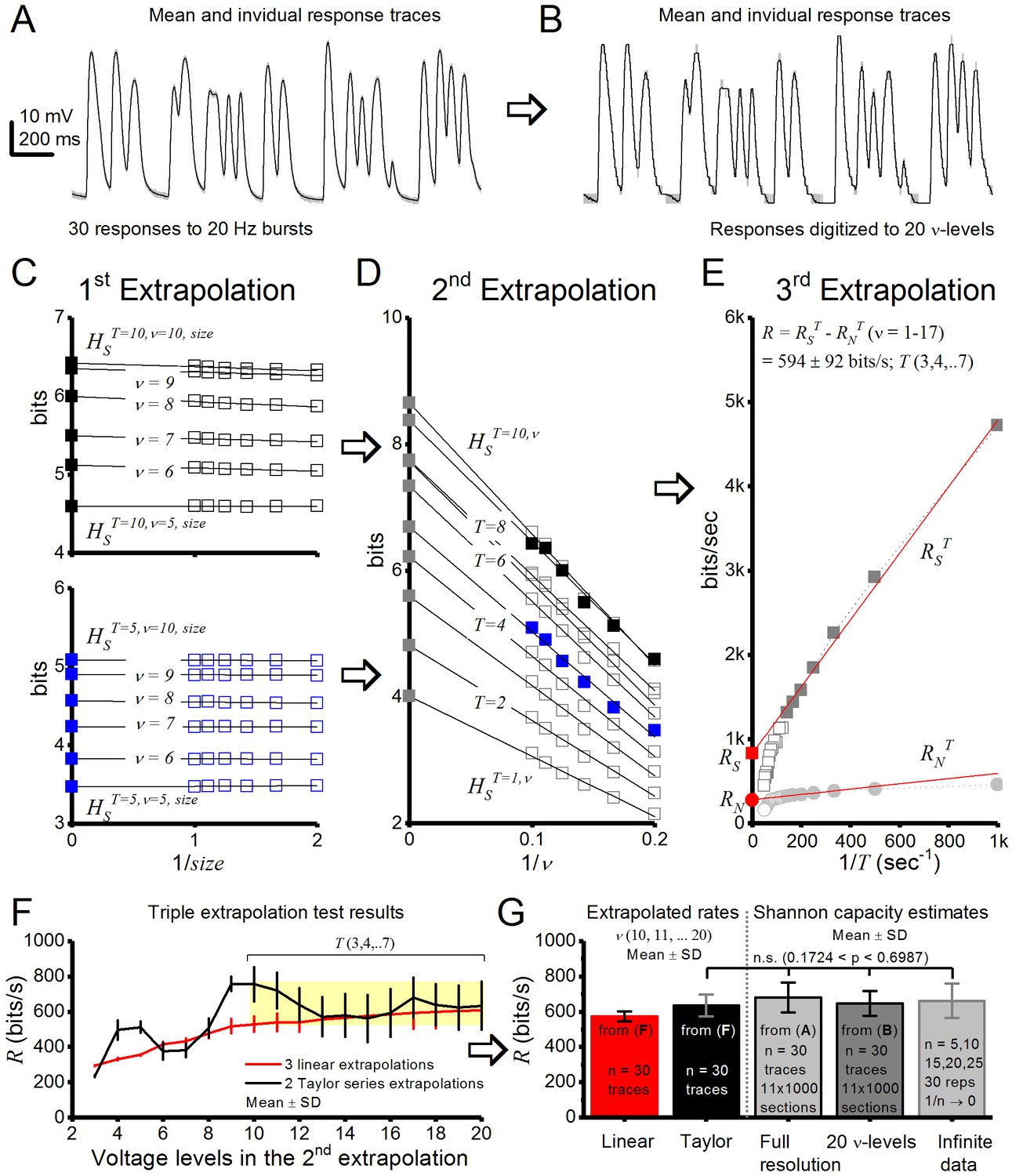
Using triple extrapolation method to estimate entropy rate, RS, noise entropy rate, RN, and information transfer rate, R, of photoreceptor output to 20 Hz bursts. (A) Mean (black) and 30 voltage responses (light gray) of a photoreceptor to a 2-s-long bursty light intensity time series. (B), The responses were digitized to 2–20 voltage levels, ν; shown for 20 levels. Entropy, HS, and noise entropy HN, are calculated for T-letters-long words, in which each 1-ms-long letter is a voltage level, ν, as explained previously (Juusola and de Polavieja, 2003). (C) first extrapolation to infinite data size. Entropies of the 10 letter words (top) and five letter words (bottom) for 5–10 voltage levels fitted with linear trends. Thus, HSTT = 10,ν and HSTT = 5,ν (black and blue ■, respectively, for ν = 5–10) are obtained from extrapolation of HSTT = 10,ν,size and HSTT = 5,ν,size for size → ∞ (1/size → 0). Here, the probability of 5 letter words is similar for 50–100% of data so size corrections in HSTT = 5,ν are minute, but for 10 letter words size corrections impact HSTT = 10,ν slightly more. (D) second extrapolation to infinite voltage levels. HST,v is shown for words of 1–10 letters, each fitted with its linear trend. HST (gray ■s for T = 5–10) is obtained from the extrapolation of HST,v when ν → ∞ (1/ν → 0); HST = 5 = blue ■; HST = 10 = black ■. (E) third extrapolation. Entropy rates obtained from extrapolations to infinitely long words. The total entropy rate, RS (red ■), is obtained from a linear extrapolation when T → ∞ (1/T → 0). RN (red ●) for the same data. Both RS and RN collapse to 0 when the data are inadequate to provide a satisfactory extrapolation of HST and HNT for long words and high voltage resolutions. The graph, however, shows enough linearly aligned points for good estimations of RS, RN, and R. (F) Effect of the number of voltage levels v used in the second extrapolation on R. For v ≥ 8, the first point for the second extrapolation is the fifth voltage level. Linear fits (red) and second-order Taylor series (black) give similar estimates (<10% difference) when v = 10–20 for these data. (G) Average R estimates obtained from linear (red) or second-order Taylor series (black) fits by the triple extrapolation method (Eq. 4) and from Shannon equation (Eq. 1). These estimates for data in (A) are similar. For 20 voltage level data (B), the mean Shannon capacity estimate is only ∼2–5% less than the mean estimates for the full response waveforms with n = 30 trials or when extrapolated to infinite data (1/n → 0), implying consistency in these estimation methods.
Figure 3
Model output is realistic over the whole encoding range.
(A–B) Simulated responses of a stochastic Drosophila R1-R6 model to the tested light stimuli show similar response dynamics to the corresponding real recordings (cf. Figure 1 and Figure 1—figure supplement 1). The model has 30,000 microvilli (sampling units) that convert absorbed photons to quantum bumps (samples). Simulations at each background (BG) were set for the mean light level (effective or absorbed photons/s) that generated responses with the maximum information transfer (Appendix 2). These effective light levels should correspond to the optimal photomechanical screening throughput (by intracellular pupil mechanism and photomechanical rhabdomere contractions, Appendix 7), which minimize saturation effects (refractory microvilli) on a Drosophila photoreceptor; see Figure 4. Notice that the model had no free parameters - it was the same in all simulations and had not been fitted to data. Thus, these macroscopic voltage responses emerged naturally as a by-product of refractory information sampling by 30,000 microvilli. Yellow box: maximum information responses. Vertical dotted rectangle (orange square) and horizontal rectangle (black circle): responses for contrast and bandwidth analyses in Figure 4.
-
Figure 3—source data 1
Simulated voltage responses of a biophysically realistic R1-R6 photoreceptor model to very bright 20 Hz, 50 Hz, 100 Hz, 200 Hz and 500 Hz bursty light stimuli at BG0 (darkness).
- https://doi.org/10.7554/eLife.26117.015
-
Figure 3—source data 2
Simulated voltage responses of a biophysically realistic R1-R6 photoreceptor model to very bright 20 Hz, 50 Hz, 100 Hz, 200 Hz and 500 Hz bursty light stimuli at BG0.5.
- https://doi.org/10.7554/eLife.26117.016
-
Figure 3—source data 3
Simulated voltage responses of a biophysically realistic R1-R6 photoreceptor model to very bright 20 Hz, 50 Hz, 100 Hz, 200 Hz and 500 Hz GWN light stimuli at BG1.
- https://doi.org/10.7554/eLife.26117.017
-
Figure 3—source data 4
Simulated voltage responses of a biophysically realistic R1-R6 photoreceptor model to very bright 20 Hz, 50 Hz, 100 Hz, 200 Hz and 500 Hz GWN light stimuli at BG1.5.
- https://doi.org/10.7554/eLife.26117.018
Figure 4

Model encodes light information realistically.
Encoding capacity of a stochastic photoreceptor model peaks to high-contrast bursts with 100 Hz cut-off, much resembling that of the real recordings (cf. Figure 2). (A) Inserts show simulations for the bursty input patterns of similar high contrast values (left) that drove its responses (outputs) with maximum information transfer rates. Output signal-to-noise ratios peaked for 20 Hz bursts (red), but was the broadest for 100 Hz bursts (yellow). Signal-to-noise ratio rose with stimulus contrast (right). (B) The corresponding probability density functions show that 100 Hz bursts evoked responses with the broadest Gaussian amplitude distribution (yellow). Only responses to low-frequency bursts (20–50 Hz) deviated from Gaussian (skewed). (C) Information transfer of the model output reached its global maximum (infomax) of 632.7 ± 19.8 bits/s (yellow) for 100 Hz (left) bursts (right). Corresponding information transfer for Gaussian white-noise stimuli was significantly lower. (D) Encoding efficiency peaked for low-frequency stimuli (left), decaying gradually with increasing contrast. For details see Appendix 2.
Figure 5 with 1 supplement
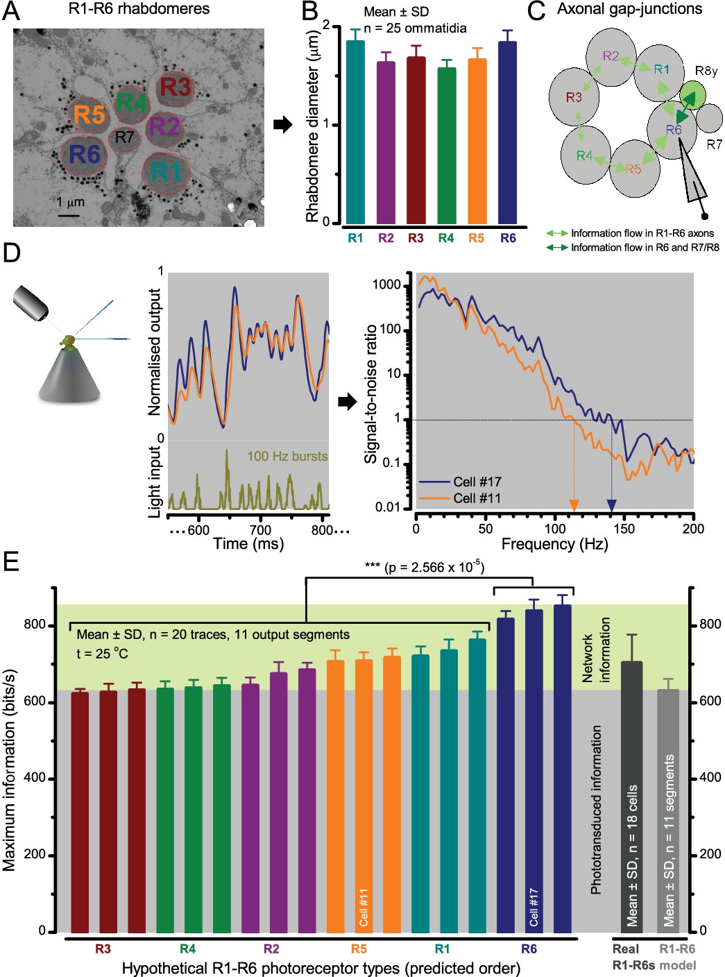
Each R1-R6 has a different diameter rhabdomere and network connections, and thus should extract different amounts of information from the same stimulus.
(A) Electron micrograph of an ommatidium, showing R1-R7 rhabdomeres with characteristic cross-sectional area differences. (B) R1 and R6 rhabdomeres are always the largest and R4 the smallest (statistics in Appendix 5, Appendix 4—table 1). (C) R6 can receive ~ 200 bits/s of network information through axonal gap-junctions from R7/R8 (Wardill et al., 2012) in the lamina about local light changes - due to their neural superposition. Gap-junctions between R1-R6 axons and synapses (Zheng et al., 2006; Rivera-Alba et al., 2011) in the lamina redistribute information (Appendix 2). (D) R1-R6s’ response waveforms and frequency range varied cell-to-cell; as evidenced by the recording system’s low noise and the cells’ high signal-to-noise ratios (~1,000). Here, Cell #17 encoded 100 Hz bursts reliably until ~ 140 Hz, but Cell #11 only until ~ 114 Hz. See also Figure 5—figure supplement 1. (E) Maximum information (for 100 Hz bursts) of 18 R1-R6s, grouped in their predicted ascending order and used for typifying the cells. Because R6s’ rhabdomeres are large (B), and their axons communicate with R7/R8 (C), the cells with the distinctive highest infomax were likely this type (blue). Conversely, R3, R4 and R2 rhabdomeres are smaller and their axons furthest away from R7/R8, and thus they should have lower infomaxes. Notably, our photoreceptor model (Song et al., 2012) (grey), which lacked network information, had a similar infomax. The mean infomax of the recordings was 73 bits/s higher than the simulation infomax.
Figure 5—figure supplement 1
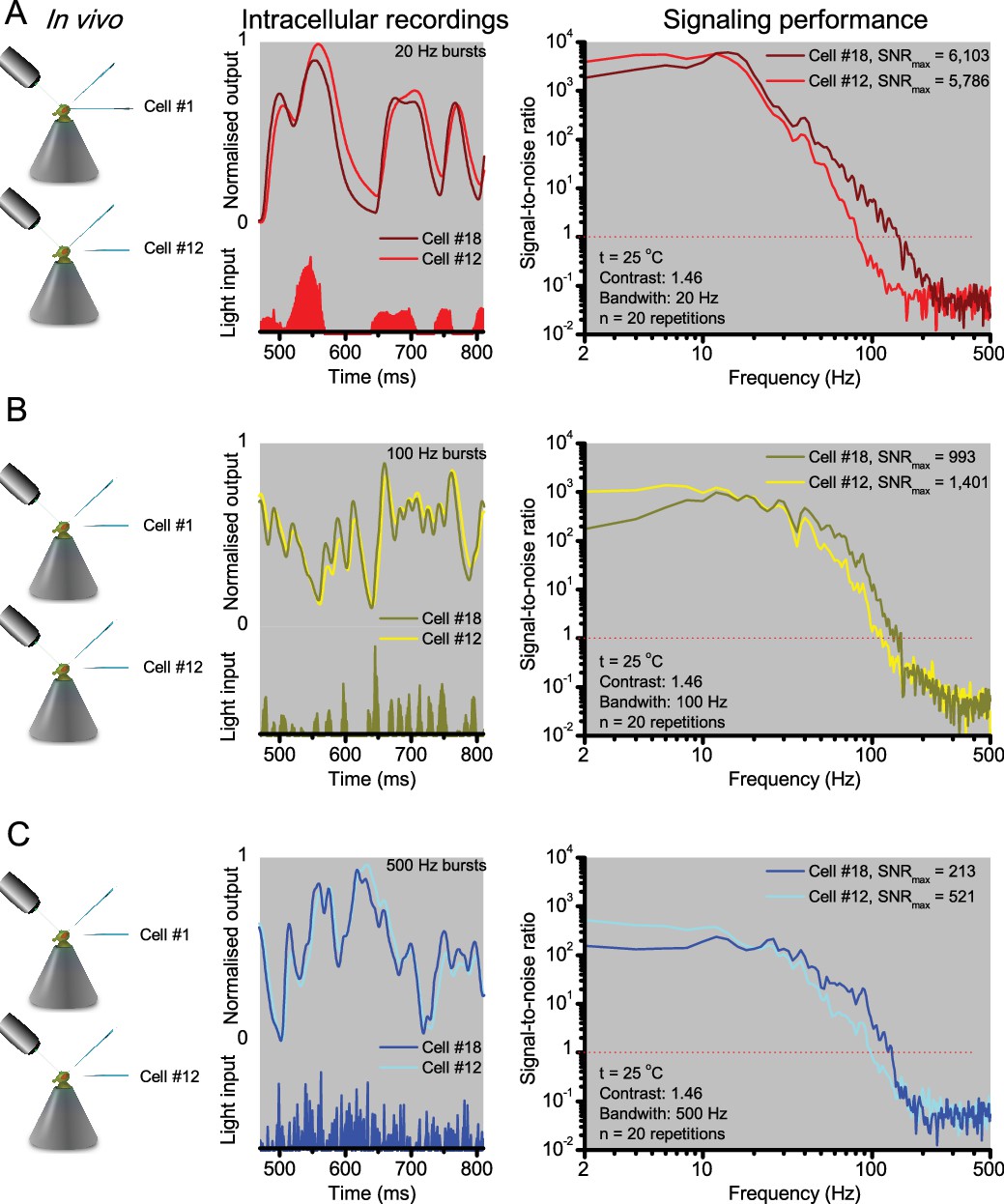
R1-R6 photoreceptors’ response waveforms and frequency range of reliable encoding vary cell-to-cell, and this variation does not reflect recording quality.
Intracellular responses to the same repeated stimuli recorded in vivo from two different R1-R6 photoreceptors (Cell #18 and Cell #12) in two wild-type Drosophila. (A) 20 Hz light bursts drove both cells vigorously, but the output of Cell #18 rose and decayed faster. Both outputs had maximum signal-to-noise ratios (SNRmax) >5,000, but because of its faster response dynamics Cell #18 encoded better high stimulus frequencies (B-C) for 100 and 500 Hz light bursts, respectively, Cell #12’s output had a higher SNRmax but again laged behind Cell #18’s output. The corresponding information transfer rate estimates, Routput, for Cell #18 were 787 bits/s (20 Hz bursts), 850 bits/s (100 Hz) and 625 bits/s (500 Hz) and for Cell #12: 569 bits/s (20 Hz), 711 bits/s (100 Hz) and 503 bits/s (500 Hz).
Figure 6 with 1 supplement
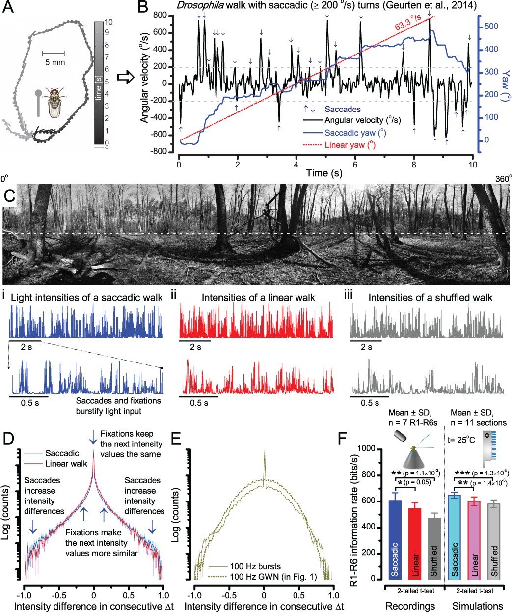
A Drosophila’s saccadic turns and fixation periods generate bursty high-contrast time series from natural scenes, which enable R1-R6 photoreceptors (even when decoupled from visual selection) to extract information more efficiently than what they could by linear or shuffled viewing.
(A) A prototypical walking trajectory recoded by Geurten et al. (2014) (B) Angular velocity and yaw of this walk. Arrows indicate saccades (velocity ≥ |±200| o/s). (C) A 360o natural scene used for generating light intensity time series: (i). ) by translating the walking fly’s yaw (A–B) dynamics on it (blue trace), and (ii) by this walk’s median (linear: 63.3 o/s, red) and (iii) shuffled velocities. Dotted white line indicates the intensity plane used for the walk. Brief saccades and longer fixation periods ‘burstify’ light input. (D) This increases sparseness, as explained by comparing its intensity difference (first derivative) histogram (blue) to that of the linear walk (red). The saccadic and linear walk histograms for the tested images (Appendix 3; six panoramas each with 15 line-scans) differed significantly: Peaksac = 4478.66 ± 1424.55 vs Peaklin = 3379.98 ± 1753.44 counts (mean ± SD, p=1.4195 × 10⁻³², pair-wise t-test). Kurtosissac = 48.22 ± 99.80 vs Kurtosislin = 30.25 ± 37.85 (mean ± SD, p=0.01861, pair-wise t-test). (E) Bursty stimuli (in Figure 1, continuous) had sparse intensity difference histograms, while GWN (dotted) did not. (F) Saccadic viewing improves R1-R6s’ information transmission, suggesting that it evolved with refractory photon sampling to maximize information capture from natural scenes. Details in Appendix 3.
Figure 6—figure supplement 1
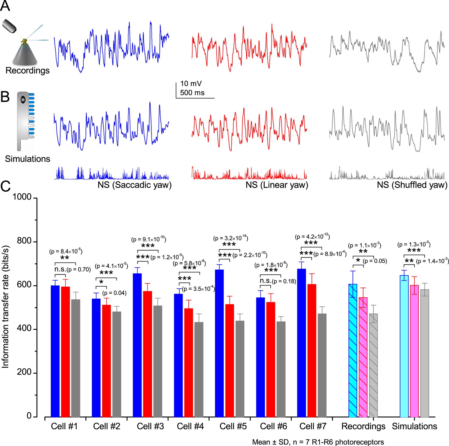
Drosophila R1-R6 photoreceptors generate responses with higher information transfer rates to saccadic (bursty) naturalist light intensity time series (NS) than to corresponding linear or shuffled stimulation.
(A) Mean intracellular voltage responses of a R1-R6 photoreceptor to Naturalistic light intensities that have been modulated by saccadic (blue), linear (red) and shuffled (gray) yaw signals. (B) Simulations of biophysically realistic Drosophila R1-R6 photoreceptor model (Appendix 1) to the same stimuli. (C) Mean information transfer rates of seven R1-R6 photoreceptor outputs to the same stimuli and their population means. These information rates are further compared to the corresponding model output rates. Note that every photoreceptor sampled most information from the NS with saccadic modulation.
Figure 7 with 2 supplements
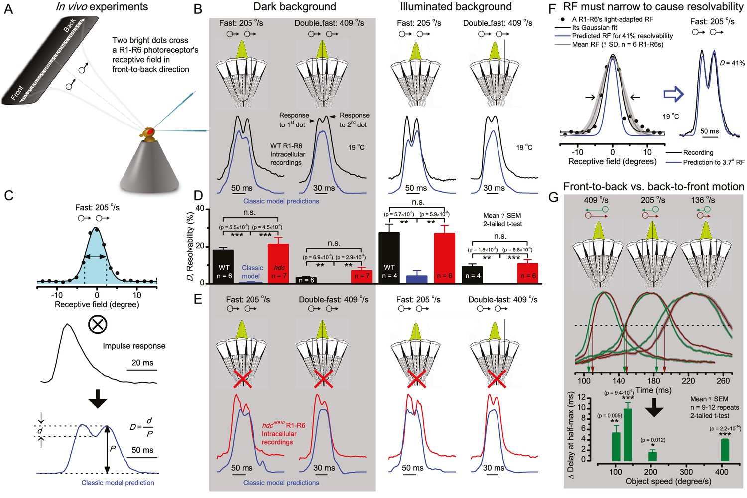
Photoreceptors resolve dots at saccadic velocities far better than the classic models.
(A) 25-light-point stimulus array centered at a R1-R6’s receptive field (RF). Each tested photoreceptor saw two bright dots, 6.8o apart, travelling fast (205 o/s) or double-fast (409 o/s) in front-to-back direction. (B) Responses (black), both at dark (left) or illuminated backgrounds (right), characteristically showed two peaks. In contrast, the corresponding classic model simulations (blue) rarely resolved the dots. (C) In the simulations, each photoreceptor’s receptive field (or its Gaussian fit) was convolved with its impulse response (first Volterra kernel). The resolvability, D, of the recordings and simulations, was determined by Raleigh criterion. (D) Recordings outperformed simulations. (E) hdcJK910 R1-R6s (red), which lacked the neurotransmitter histamine, and so network modulation, resolved the dots as well as the wild-type, indicating that the recordings’ higher resolvability was intrinsic and unpredictable by the classic models (Appendix 6). (F) To resolve the two dots as well as a real R1-R6 does in light-adaptation, the model’s acceptance angle (∆ρ) would need to be ≤3.70o (blue trace); instead of its experimentally measured value of 5.73 (black; the narrowest ∆ρ. The population mean, grey, is wider). (G) Normalized responses of a typical R1-R6 to a bright dot, crossing its receptive field in front-to-back or back-to-front at different speeds. Responses to back-to-front motions rose and decayed earlier, suggesting direction-selective encoding. This lead at the half-maximal values was 2–10 ms. See Appendixes 4 and 6.
Figure 7—figure supplement 1
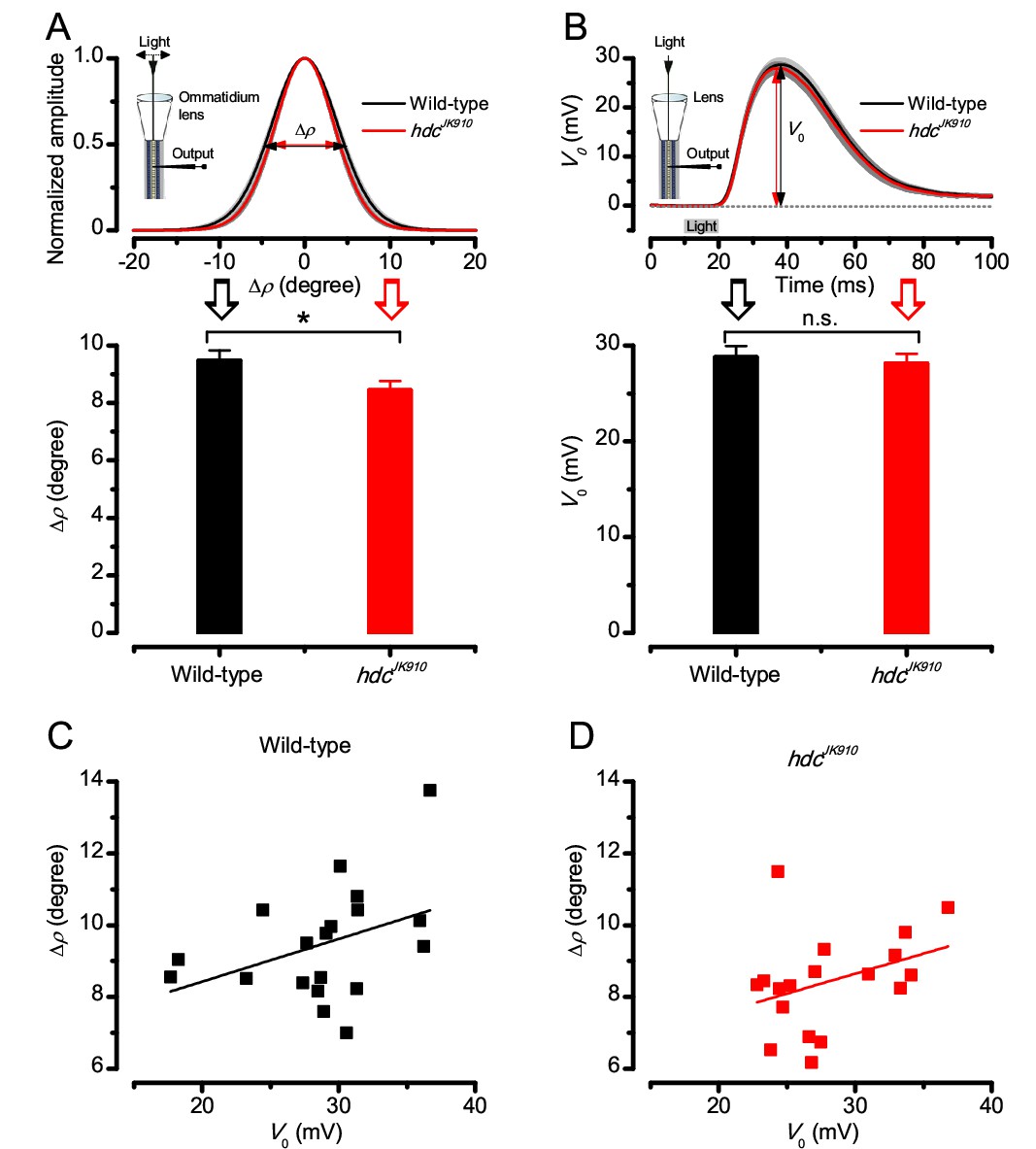
Dark-adapted wild-type and hdcJK910 R1-R6s’ acceptance angles differ marginally.
The receptive field of each tested cell was estimated as in Appendix 4, Appendix 4—figure 2. (A) Dark-adapted wild-type photoreceptors’ receptive fields (above), shown as the mean of their Gaussian fits (black), were ~11% wider than those of hdcJK910 photoreceptors (red). Their receptive field sizes (below) were quantified by the corresponding half-maximum widths, giving the mean acceptance angles: ∆ρwild-type = 9.47 ± 0.36°; ∆ρhdc = 8.44 ± 0.32°; p=0.0397, two-tailed t-test. (B) Wild-type and mutant photoreceptors’ peak responses (above), evoked by a sub-saturating 10 ms light flash (grey bar) at the center of the receptive field, showed similar dynamics and amplitudes, V0 (below). V0wild-type = 28.77 ± 1.19 mV; V0hdc = 28.11 ± 1.03 mV; p=0.67, two-tailed t-test. This indicates that hdcJK910 phototransduction is functionally intact and wild-type-like. See also (Dau et al., 2016). (C) Linear correlation between ∆ρ and V0 of dark-adapted wild-type photoreceptors. Adjusted R-squared = 0.1043. (D) Linear correlation between ∆ρ and V0 of dark-adapted hdcJK910 photoreceptors. Adjusted R-squared = 0.072. (A-D) nwild-type = 19; nhdc = 18. (A, B) Mean ± SEM; two-tailed t-test.
Figure 7—figure supplement 2
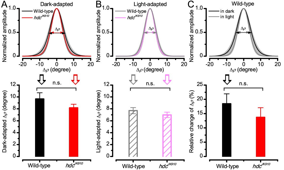
Light-adaptation narrows wild-type and hdcJK910 R1-R6s’ receptive fields similarly.
Comparing wild-type and hdcJK910 photoreceptors, of which receptive fields were assessed in both the dark- and light-adapted states. (A) Their dark-adapted and (B) and light-adapted ∆ρ values were similar. Dark-adapted: ∆ρwild-type = 9.65 ± 1.06°; ∆ρhdc = 8.16 ± 0.62°; p=0.258, two-tailed t-test. Light-adapted: ∆ρwild-type = 7.7 ± 0.52°; ∆ρhdc = 6.98 ± 0.46°; p=0.323, two-tailed t-test. (C) Predictably, their receptive fields narrowed during light-adaptation (only wild-type shown). The relative changes between the two adaptation states between were statistically similar in wild-type and hdcJK910 photoreceptors. Relative changes, calculated as . Cwild-type = 18.44 ± 3.5%; Chdc = 13.68 ± 3.37%, p=0.347, two-tailed t-test. A-C: Mean ± SEM; nwild-type = 6; nhdc = 8 cells.
Figure 8 with 1 supplement
Microsaccadic rhabdomere contractions and refractory photon sampling improve visual resolution of moving objects.
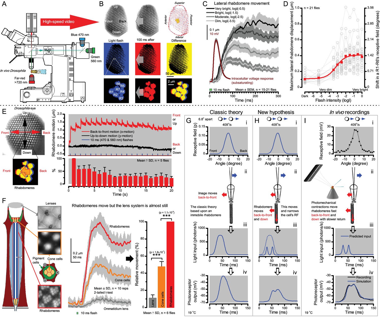
(A) High-speed videos showed fast lateral R1-R7 rhabdomere movements to blue/green flashes, recorded under far-red illumination that Drosophila barely saw (Wardill et al., 2012). (B) Rhabdomeres moved inside those seven ommatidia (up-right: their pseudopupil), which faced and absorbed the incident blue/green light, while the others reflected it. Rhabdomeres moved frontwards 8–20 ms after a flash onset, being maximally displaced 70–200 ms later, before returning. (C) Movements were larger and faster the brighter the flash, but slower than R1-R6s’ voltage responses. (D) Movements followed R1-R6s’ logarithmic light-sensitivity relationship. Concurrently, given the ommatidium optics (Stavenga, 2003b; Gonzalez-Bellido et al., 2011), R1-R6s’ receptive fields (RFs) shifted by 0.5–4.0o. (E) Rhabdomeres moved along the eye’s horizontal (red) axis, with little vertical components (black), adapting to ~ 30% contractions in ~ 10 s during 1 s repetitive flashing. (F) Moving ommatidium structures. Cone and pigment cells, linking to the rhabdomeres by adherens-junctions (Tepass and Harris, 2007), formed an aperture smaller than the rhabdomeres’ pseudopupil pattern. Rhabdomeres moved ~ 2 times more than this aperture, and ~ 10 times more than the lens. (G–H) Simulated light inputs and photoreceptor outputs for the classic theory and new ‘microsaccadic sampling’-hypothesis when two dots cross a R1-R6’s RF (i) front-to-back at saccadic speeds. (G) In the classic model, because the rhabdomere (ii) and its broad RF (i) were immobile (ii), light input from the dots fused (iii), making them neurally unresolvable (iv). (H) In the new model, with rhabdomere photomechanics (ii) moving and narrowing its RF (here acceptance angle, ∆ρ, narrows from 8.1o to 4.0o), light input transformed into two intensity spikes (iii), which photoreceptor output resolved (iv). (I) New predictions matched recordings (Figure 8—figure supplement 1). Details in Appendixes 7–8.
Figure 8—figure supplement 1
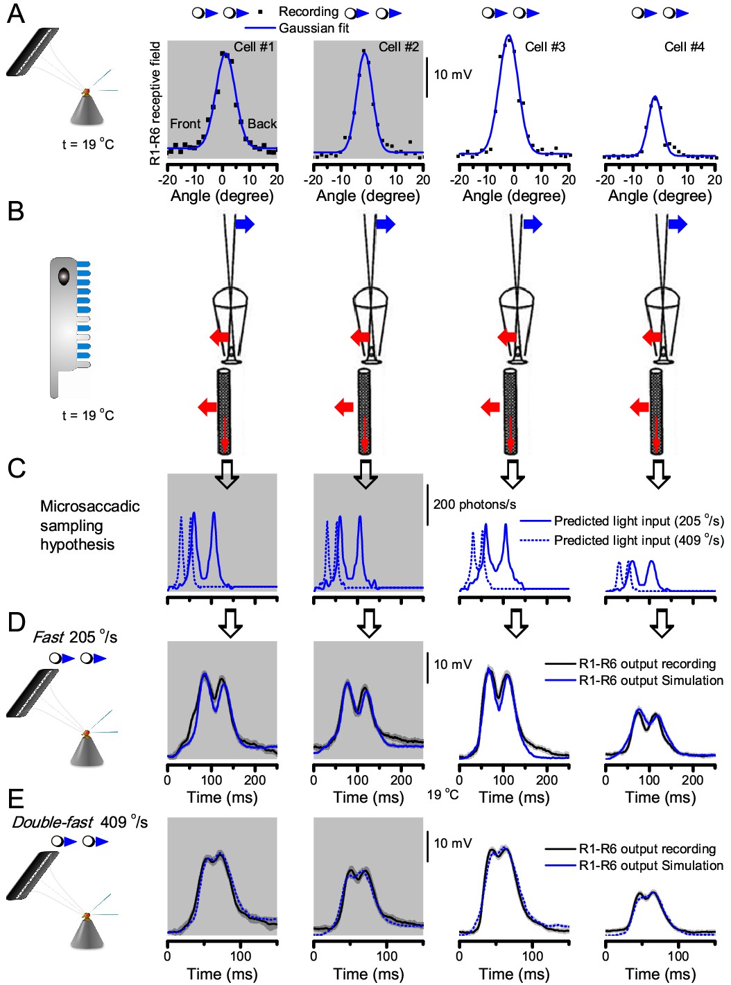
Microsaccadic sampling hypothesis predicts realistic voltage output to two bright dots crossing a R1-R6’s receptive field in saccadic speeds.
(A) Receptive fields of four R1-R6 photoreceptors, measured with 25 light point stimulator (Appendix 4). (B) Microsaccadic sampling hypothesis predicts that because the rhabdomeres move photomechanically, the photoreceptors’ receptive fields move in the opposite direction and narrow transiently (acceptance angles, ∆ρ, change from 8.2 to 9.5o to 3.5–4.5o). (C) The resulting light input for each tested photoreceptor was predicted from its measured receptive field in (A) by the microsaccadic sampling hypothesis. (D and E) These inputs then drove our biophysically realistic R1-R6 model, predicting the photoreceptor voltage output, which was compared to the corresponding real recordings. The simulated R1-R6 output closely resembled the recorded R1-R6 output of the same cells to saccadic two dot stimuli.
Figure 9 with 1 supplement
‘Microsaccadic sampling’ hypothesis predicts visual hyperacuity.
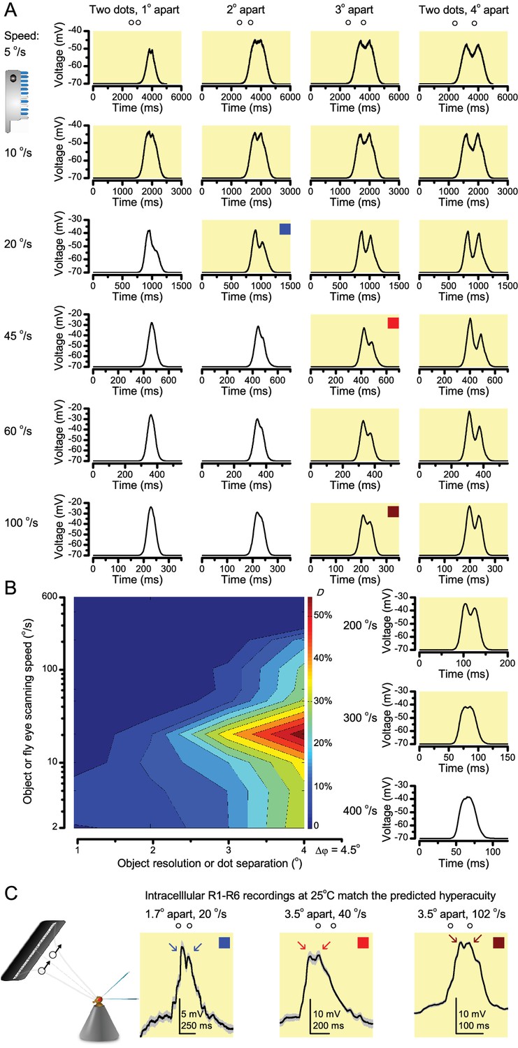
(A) Simulated R1-R6 output to two dots, at different distances apart, crossing the photoreceptor’s receptive field at different speeds. The yellow backgrounds indicate those inter-dot-distances and speeds, which evoked two-peaked responses. The prediction is that the real R1-R6s could resolve (and Drosophila distinguish) these dots as two separate objects, whereas those on the white backgrounds would be seen as one object. The simulations were generated with our biophysically realistic R1-R6 model (Song et al., 2012; Song and Juusola, 2014; Juusola et al., 2015), which now included the estimated light input modulation by photomechanical rhabdomere movements (Figure 8H). (B) The resulting object resolution/speed heat-map, using the Raleigh criterion, D (Figure 7C), shows the stimulus/behavioral speed regime where Drosophila should have hyperacute vision. Thus, by adjusting its behavior (from gaze fixation to saccadic turns) to changing surroundings, Drosophila should see the world better than its compound eye’s optical resolution. (C) Intracellular R1-R6 responses resolved the two dots, which were less that the interommatidial angle (Δφ = 4.5o) apart when these crossed the cell’s receptive field at the predicted speed range. Arrows indicate the two response peaks corresponding to the dot separation. Cf. Figure 9—figure supplement 1; details in Appendixes 7–8. These results reveal remarkable temporal acuity, which could be used by downstream neurons (Zheng et al., 2006; Joesch et al., 2010; Behnia et al., 2014; Yang et al., 2016) for spatial discrimination between a single passing object from two passing objects.
Figure 9—figure supplement 1
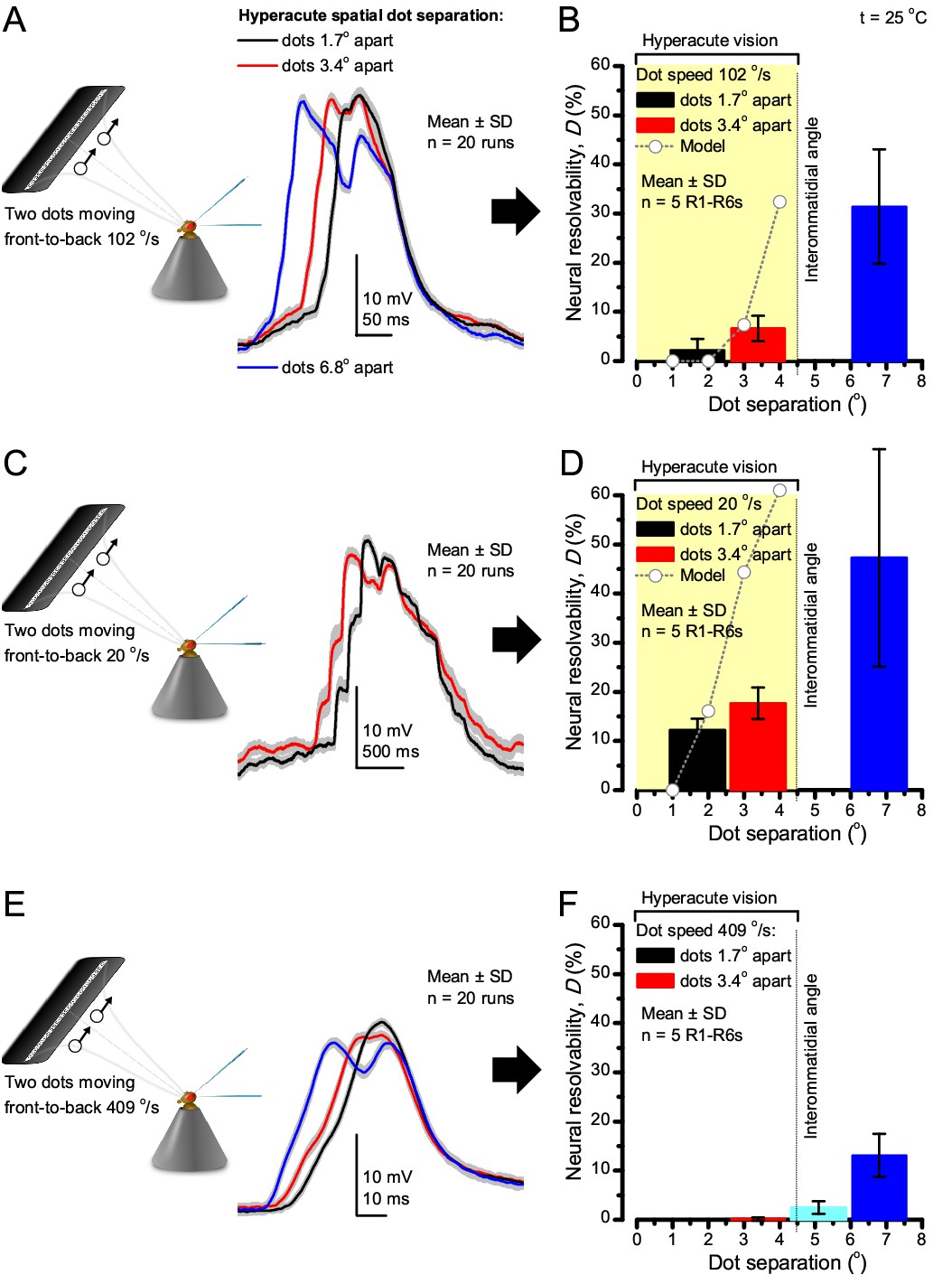
Encoding space in time - intracellular R1-R6 recordings to two bright dots crossing the receptive field show how their responses convey hyperacute spatial information in time.
25 light-point-array positioned at a R1-R6’s receptive field center, generating two bright front-to-back moving dots. (A) Characteristic responses of a R1-R6 at 25°C to the dots, 1.7, 3.4 or 6.8o apart, travelling 102 o/s in front-to-back direction. (B) Individual outputs resolved the dots, which were less than the interommatidial angle (Δφ = 4.5o) apart (yellow box); resolvability given by the Raleigh criterion (Figure 7C). Microsaccadic sampling model (Figure 9) predicted a comparable resolvability threshold (dotted line). (C) At lower dot velocities (20–50 o/s), corresponding to normal gaze fixation speeds in close-loop flight simulator experiments (Appendix 10), each R1-R6 responded to the tested hyperacute dot separations (1.7o and 3.4o) even stronger. Notice the small staircase-like steps in voltage responses. These represent light from 25 individual light-guide-ends being turned on/off in sequence to generate the moving dots, crossing the receptive field slowly (see Appendix 6). (D) At 20 o/s velocity, neural resolvability to the tested hyperacute dot separations was between 10–20%. (E) R1-R6 output to the two dots, having the same separations as above, but now moving at fast saccadic velocity (409 o/s). (F) Although, at such a high speed, R1-R6 output could not resolve the hyperacute dot separations (1.7o and 3.4o) consistently, the dots were nevertheless clearly detected when at 5.1o apart (cyan bar), which is about Δφ.
Figure 10 with 1 supplement
Optomotor behavior in a flight simulator system confirms hyperacute vision.
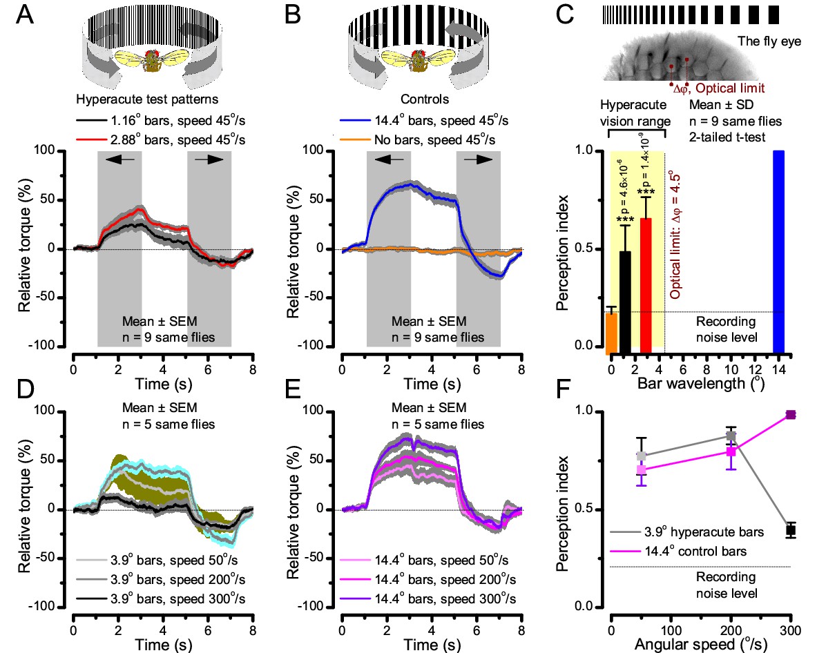
Classic open-loop experiments using high-resolution panoramas. (A) 360o hyperacute black-and-white bar panorama, with 1.16o or 2.88o wavelengths (= 0.58o and 1.44o inter-bar-distances), rotated counterclockwise and clockwise (grey, arrows) around a tethered fly, with a torque meter measuring its optomotor responses. (B) Controls: the same flies’ optomotor responses to white (no bars) and wide-bar (14.4o wavelength) rotating panoramas. (C) Every Drosophila responded to the hyperacute panoramas (wavelength < interommatidial angle, Δφ, yellow area; Figure 10—figure supplement 1), but not to the white panorama (orange), which thus provided the recording noise level. The flies optomotor responses were the strongest to the wide-bar panorama (perception index = 1). As the flies’ optomotor responses followed the rotation directions consistently, irrespective of the tested bar wavelengths, the hyperacute visual panorama did not generate perceptual aliasing. (D) Optomotor responses of five flies to hyperacute panorama with 3.9o wavelength, rotating at 50o/s and saccadic speeds of 200 and 300o/s. (E) Control responses of the same flies to 14.4o wavelength panorama at the same speeds. (F) The flies’ ability to follow hyperacute panorama reduces dramatically when the stimulation approaches the photoreceptors’ predicted acuity limit, which for ~4o point resolution is just over 300o/s (cf. Figure 9A). Details in Appendix 10.
Figure 10—figure supplement 1
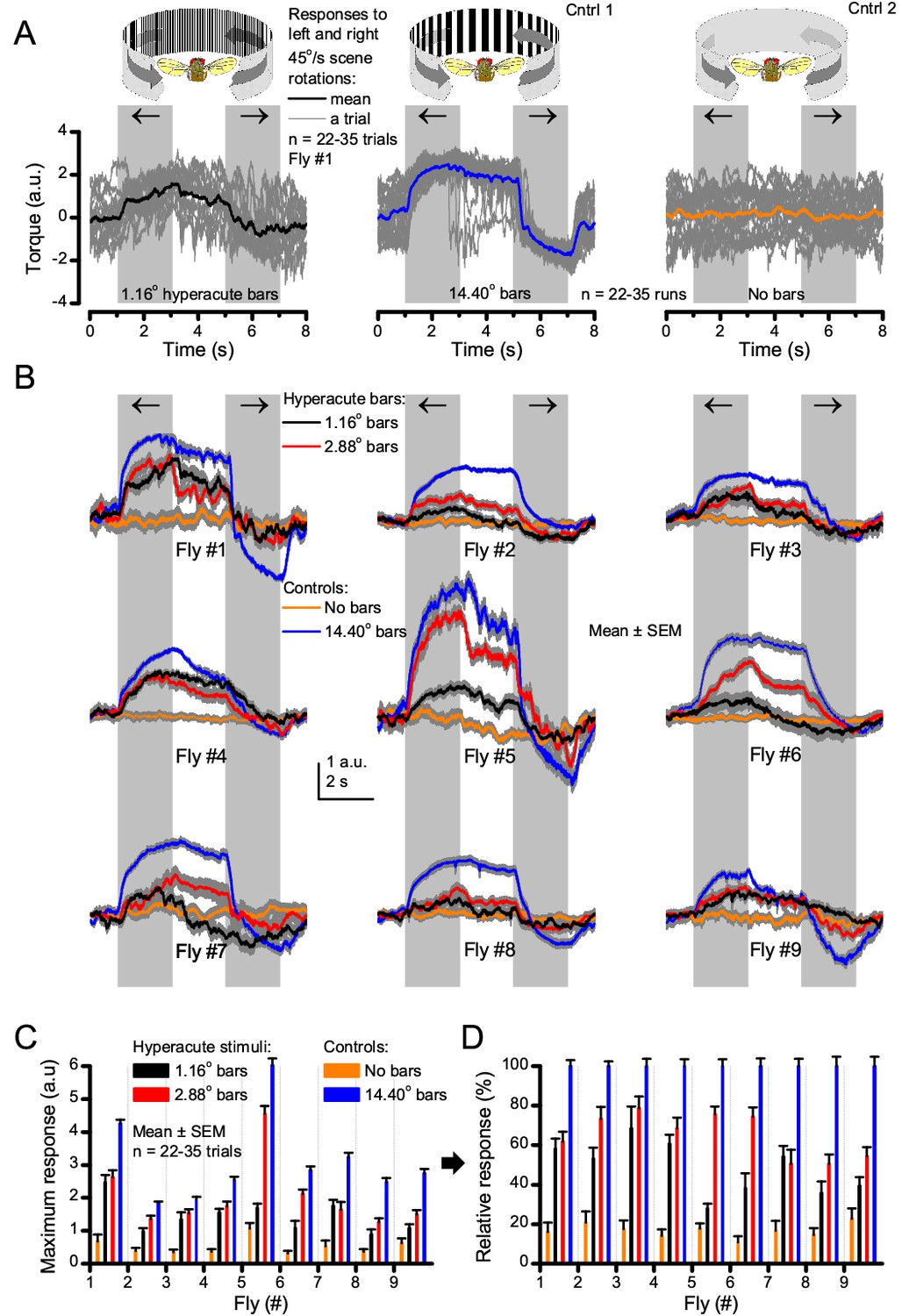
Optomotor behavior in a flight simulator system demonstrates that Drosophila see hyperacute visual patterns.
(A) 22–35 individual optomotor responses (thin grey traces) and their mean (think trace) of the same tethered fly to 45o/s clockwise and counterclockwise panoramic field rotations (light grey sections), having a full wavelength of 1.16o (left, black) or 14.40o (center, blue), or no-bar (right, orange) stimuli. (B) Every tested fly (n = 9) responded to hyperacute (<Δφ ~4.5o) bar stimuli (1,16o and 2.88o, red; having 0.58o and 1.44o inter-bar-distances, respectively) consistently. (C) Their maximum (peak-to-peak) responses to the hyperacute stimuli and the no-bar and coarse-bar controls. (D) The relative response strength to the hyperacute stimuli varied between 30–80% of the maximum responses to the coarse-bar stimulus.
Appendix 1—figure 1
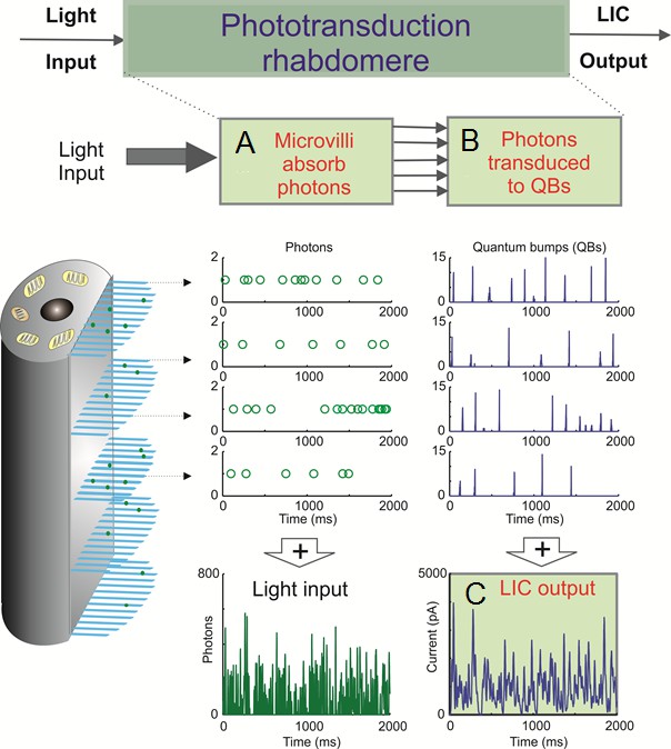
Schematic of the biophysically realistic Drosophila R1-R6 model, which mimics phototransduction by transducing light input (a dynamic flux of photons) into macroscopic output, light-induced current (LIC).
The model is modular, containing four parts, three of which are shown here. Phototransduction occurs within a photoreceptor’s light-sensitive part, the rhabdomere, which contains 30,000 photon sampling units, microvilli (blue bristles). Each microvillus contains a full phototransduction cascade reactions, and can transduce single photon energies (green dots) into unitary responses, quantum bumps (QB or samples) of variable amplitudes. (A) In the first module, 30,000 microvilli sample incoming photons. The light input, as photons/s, is randomly distributed over them (each row of open circles indicate photons being absorbed by a single microvillus). (B) In the second module, the successfully absorbed photons in each microvillus are transduced into QBs (a row of unitary events). In each microvillus, the success of transducing a photon into a QB depends upon the refractoriness of its phototransduction reactions. This means that a microvillus cannot respond to the next photons until its phototransduction reactions have recovered from the previous photon absorption, which takes about 50–300 ms. The photons hitting a refractory microvillus cannot evoke QBs, but will be lost. (C) In the third module, QBs from all the microvilli then integrate the dynamic macroscopic LIC. Conversely, the light input (green trace) can be reconstructed by adding up all the photons distributed across the 30,000 microvilli.
Appendix 1—figure 2
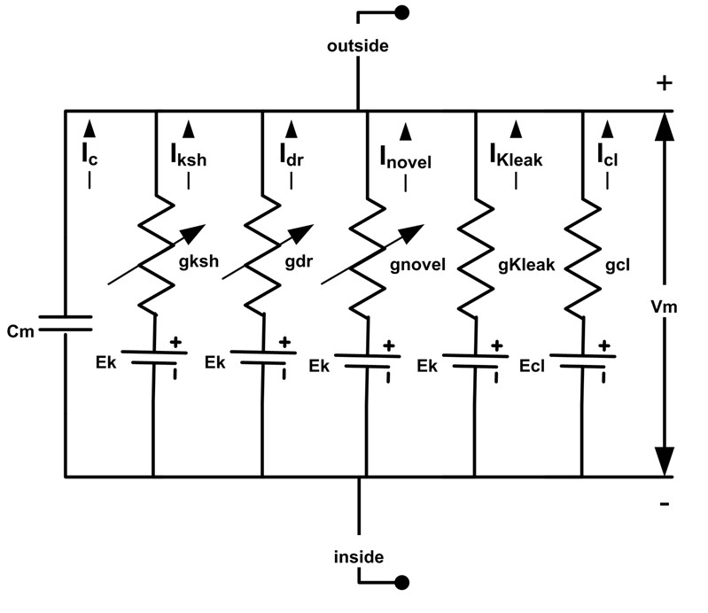
Drosophila R1-R6 photoreceptor membrane’s electrical circuit (HH-model).
A photoreceptor’s membrane potential, Vm, is the difference between the negative inside (intracellular) and positive outside (extracellular) voltages. Vm can be calculated, using Hodgkin-Huxley formalism, whereupon, a photoreceptor membrane is modelled as a capacitor, Cm, voltage-gated channels as voltage-regulated conductances, g, leak channels as fixed conductances, reversal potentials for different ion species as DC-batteries. Abbreviations: Iksh: Shaker; Idr, delayed rectifier; Inovel, novel K+; Kleak: K+ leak; Icl, chloride leak currents. The used deterministic Drosophila photoreceptor HH-model is adapted from (Niven et al., 2003; Vahasoyrinki et al., 2006).
Appendix 2—figure 1
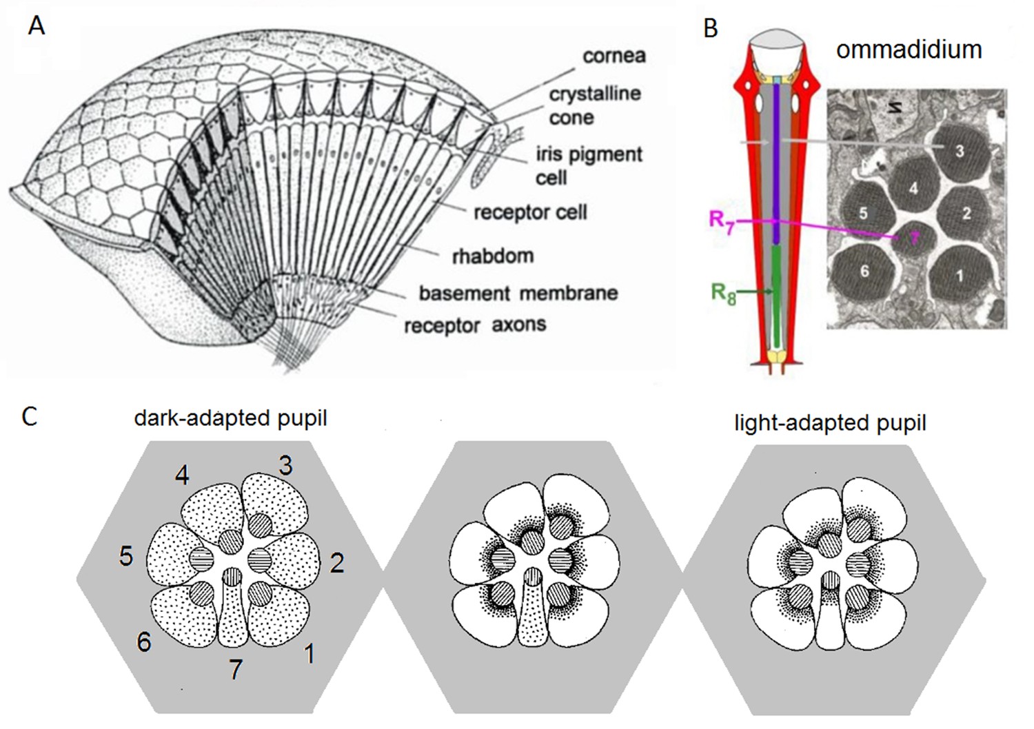
Compound eye and photoreceptors’ intracellular pupil mechanism.
(A) Drosophila eyes are composed of about 800 modular units, ommmadia. (B) Each ommatidium contains a lens system and underneath it eight photoreceptor cells: the outer receptors, R1-R6, and the inner receptors, R7/R8. In the electron micrograph, which numbers each cell’s rhabdomere (light sensitive part), R8 is not shown because it lies directly below R7. (C) Schematic of the intracellular pupil mechanism. Left: During dark-adaptation, screening pigments (small dots) are scattered in the R1-R7 somata. Middle: R1-R6 light-adapted. Blue-green bright light drives the screening pigment migration towards the R1-R6 rhabdomeres (central discs, containing 30,000 microvilli, photon sampling units, depicted as stripes in the discs), which express blue-green-sensitive Rh1-rhodopsin, as their phototransduction rises intracellular Ca2+-concentration. With the pupil closing (seen as the dark rims around the rhabdomeres), light input to the microvilli reduces. Note that R7, which expresses UV-rhodopsin, is not light-adapted and its screening pigments remain scattered. Right: All photoreceptors light-adapted. Bright UV-light closes all pupils because R7s express UV-sensitive Rh3- and Rh4-rhodopsins, and in R1-R6s’ Rh1-rhodopsin is electrochemically coupled to UV-sensitive sensitizing pigment. Redrawn and modified from (Franceschini and Kirschfeld, 1976; Elyada et al., 2009).
Appendix 2—figure 2
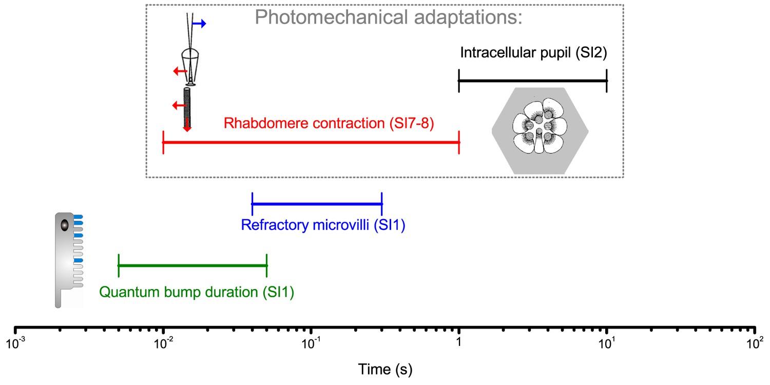
Different temporal ranges of a Drosophila R1-R6 photoreceptor’s intrinsic light adaptation mechanisms.
Photomechanical adaptations, such as light-induced intracellular screening pigment migration (pupil mechanism, black; see Appendix 2—figure 1) and rhabdomere contractions (red; see Appendix 7), operate with refractory photon sampling by 30,000 microvilli (blue) and their quantum bump dynamics (sample duration and jitter, green; see Appendix 1) in modulating light input to a photoreceptor, and consequently its voltage output. Together these mechanisms, which work to eliminate excess photons, enable efficient encoding of behaviorally important visual information at daylight conditions (Figures 1–2) by covering a broad range of temporal light changes; with the pupil and rhabdomere contractions being slower than the photon sampling dynamics.
Appendix 2—figure 3
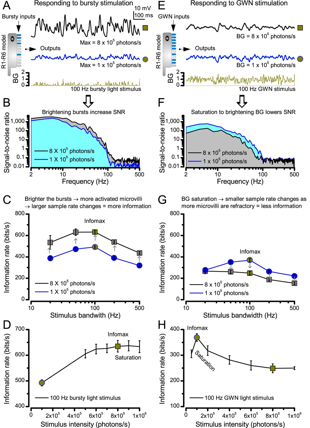
Estimating optimal light intensity for 100 Hz high-contrast bursts and Gaussian white-noise (GWN) stimuli for a R1-R6 photoreceptor’s maximal information transfer.
We hypothesize that the role of photomechanical adaptations, which include the intracellular pupil and contracting rhabdomere (Appendix 7) of a photoreceptor, is to maximize information capture of microvilli by dynamically adjusting the light input falling upon them. The left side of the figure shows how encoding of light bursts (A–D) depends upon light intensity; the right side shows the same for GWN (E–H). (A) Owing to sufficient dark periods, a photoreceptor’s sampling units (microvilli) have enough time to recover from their refractoriness even after they have responded to very bright bursts. This enables a photoreceptor to maintain a large pool of available microvilli to sum up high sample (bump) rate changes to any new incoming input, generating larger macroscopic responses to the brighter bursts (8 × 10⁵ photons/s, black) than to the less bright bursts (105 photons/s, blue). (B) Macroscopic responses with larger sample rate changes (black trace, grey area) have higher and broader signal-to-noise ratios (Song and Juusola, 2014). (C) Correspondingly, as the sample sizes (bumps) are similar to both stimuli (cf. Figure 2—figure supplement 2B), the larger responses carry a higher information transfer rate (Song and Juusola, 2014), irrespective of the tested stimulus bandwidth. (D) Therefore, a photoreceptor’s information transfer rate to bursty inputs increases with light intensity, until the sample rate changes eventually saturate at 8 × 10⁵ photons/s; when most of 30,000 microvilli become refractory (i.e. more microvilli are refractory than available to be light-activated). (E) A R1-R6 generates similar size responses to the brighter (8 × 10⁵ photons/s, black) and the less bright (105 photons/s, blue) GWN inputs. But the response to the less bright input shows more high-frequency modulation. (F) Consequently, the response to the less bright input (blue area) has higher and broader signal-to-noise ratio than the response to the brighter input (grey area). (G) This is reflected also in the photoreceptor’s information transfer rate, regardless of the GWN bandwidth. (H) Information transfer rate in macroscopic photoreceptor output to GWN stimulation saturates at 8-times less bright intensity levels than to bursts (D), reaching its maximum at 105 photons/s.
Appendix 2—figure 4
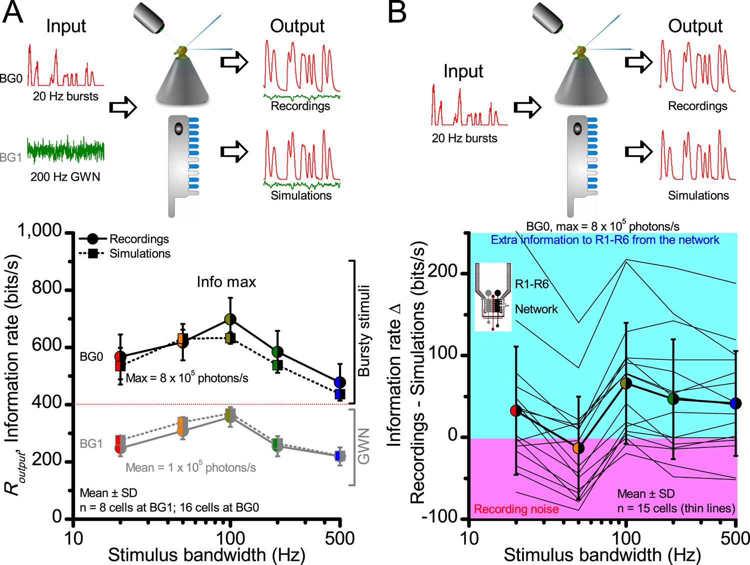
Information transfer rate estimates, Routput, of in vivo recordings and model simulations show similar encoding dynamics.
(A) Comparison of corresponding information transfer rates of R1-R6 recordings and stochastic model simulations to light bursts and Gaussian white noise (GWN) stimuli of different bandwidths. The recorded and simulated information transfer estimates correspond closely over the whole tested encoding space (cf. Figure 2—figure supplement 1 and Figure 4). (B) Their differences to light bursts help to identify extra information in the recordings, which likely comes from the lamina network (through gap-junctions (Wardill et al., 2012) and feedback synapses [Zheng et al., 2006]) to individual photoreceptors. The clear variability between different recordings from individual cells (continuous thin lines) indicates that some R1-R6s may receive up to 200–250 bits/s of information from the network, whereas others receive less (cyan background). Some recordings likely contained more instrumental/experimental noise (pink background), which could render their information transfer rates (in particular to low-frequency bursts) less than that of the model; some of this noise likely comes from low-frequency eye and photoreceptor movements (cf. Figure 2—figure supplement 2). Thick line and error bars give the average information transfer rate difference between the recordings and the model (~0–50 bits/s). The data implies that the extra network information to R1-R6s in vivo is mostly at high burst frequencies (100–500 Hz).
Appendix 2—figure 5
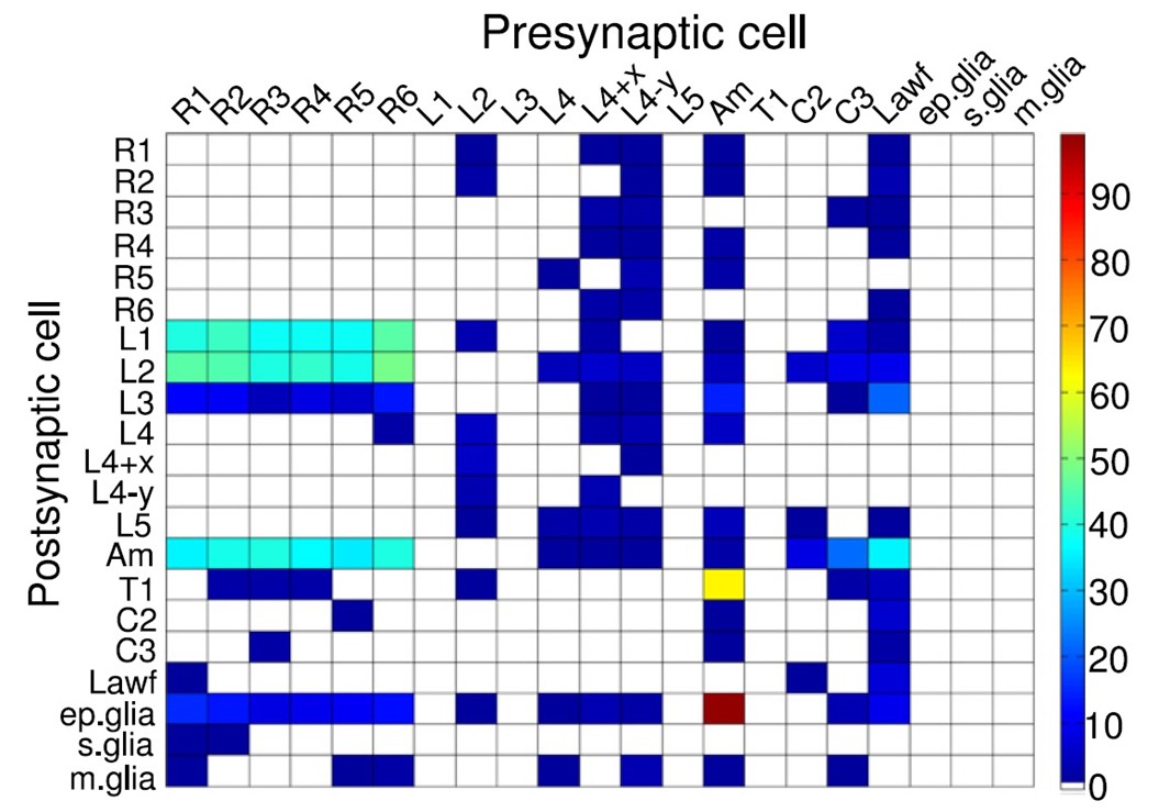
Synaptic connectivity between neurons within a lamina cartridge.
Synapse numbers color-coded as indicated by the column on the right. Large monopolar cells, L1-L5; amacrine cell, Am; C2 and C3 are retinotopic centrifugal fibers from the next synaptic processing layer, medulla. Image from (Rivera-Alba et al., 2011).
Appendix 2—figure 6
Gap-junction spread information.
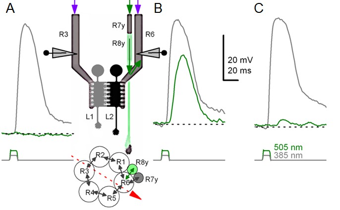
Because of axonal gap-junctions between R6 and R7/R8 photoreceptors in the lamina (Shaw, 1984; Shaw et al., 1989), R1-R6s that have been genetically engineered to express UV-sensitive Rh3-rhodopsin (‘UV-flies’) can still respond to green light by different degrees (Wardill et al., 2012). This flow of extra ‘color’- information can be readily identified in intracellular responses of different R1-R6 photoreceptors in the same ‘UV-fly’ to very bright UV (385 nm) and green-yellow (505 nm) flashes. (A) First cell responded to UV but not to green. (B) Next cell (likely R6 in the same or neighboring neuro-ommatidium) responded to both UV and green. This cell cannot be R7y/p, which are less green-sensitive, or R8y/p, which are less UV-sensitive. Inset highlights a hypothetical recording path, somewhere close to the retina/lamina border (red arrow), and gap-junctions (black arrows) between photoreceptor axons. Histaminergic L1 and L2 cells receive visual information from R1-R6 photoreceptors’ output synapses in the same neuro-ommatidium. (C) Another cell responded to UV and weakly to green-yellow. Modified from (Wardill et al., 2012).
Appendix 2—figure 7

Projected image of Sin(x2 + y2) function is used to illustrate the effect of aliasing and how stochastic variability in the sampling matrix combats aliasing effectively.
(A) Sin(x2+y2) is plotted with 0.1 resolution. (B) Under-sampling the same image by an ordered matrix leads to aliasing: ghost rings appear when the image (of the function) is sampled with 0.2 resolution. Aliasing is a critical problem, as the nervous system cannot differentiate the fake image rings from the original real image. (C) Sampling the image (A) with a random matrix may lose some of its fine resolution, due to broadband noise, but such sampling is anti-aliasing; sampling with random points at 0.2 resolution. (D) Color photoreceptor distributions across macaque (Field et al., 2010) (red, green and blue cones; left) and Drosophila retina (Vasiliauskas et al., 2011) (R7y and R7p receptors; right) show random-like sampling matrixes, suggesting that this sampling matrix sensitivity randomization would have an anti-aliasing role. (E) Crucially, by integrating and redistributing R1-R6 outputs with additional gap-junctional inputs from randomized R7/R8 color channels (Wardill et al., 2012) (D) and Appendix 2—figure 6) for each image pixel during synaptic transmission to LMCs, any broadband sampling noise should be much reduced and the R1-R6 (motion) channel’s spectral range whitened (Wardill et al., 2012). Note how LMC output peaks before the corresponding R1-R6 output. Scale bars: 10 mV / 20 ms. Sub-figure (E) is modified from (Wardill et al., 2012).
Appendix 3—figure 1
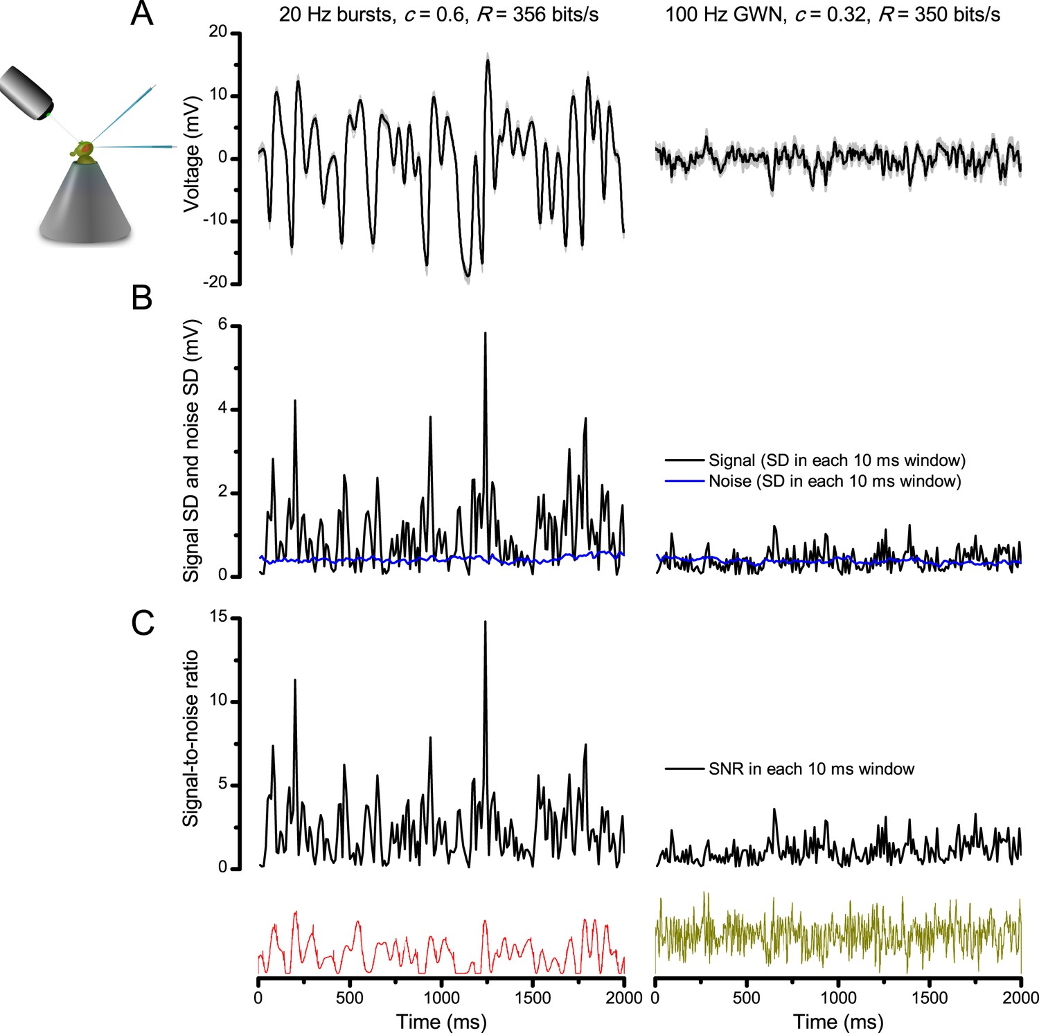
Bursts are informative.
Whilst having similar information transfer rates, the responses to bursty stimuli (left) show higher signal-to-noise ratio within brief (10–100 ms) perceptually relevant time windows than the responses to Gaussian white-noise (GWN, right). The data are from the same cell. (A) 25 intracellularly recorded voltage responses to repeated bursty and GWN light stimuli. Individual responses (superimposed) are shown in light grey and their mean in black traces. Both of these responses series carry similar information contents (~350 bits/s), as estimated by Shannon’s equation (see Equation A2.1). (B) The signal (average response) standard deviation (SD) in 10 ms windows to bursty stimulation vary much more than that to white-noise. The noise variability (blue traces) in the two sets of responses (SD in 10 ms time windows) is similar. (C) Signal-to-noise ratio is much greater in the responses to light bursts than to white-noise stimulation; it was calculated as the ratio between signal SD and noise SD, using 10 ms time resolution.
Appendix 3—figure 2
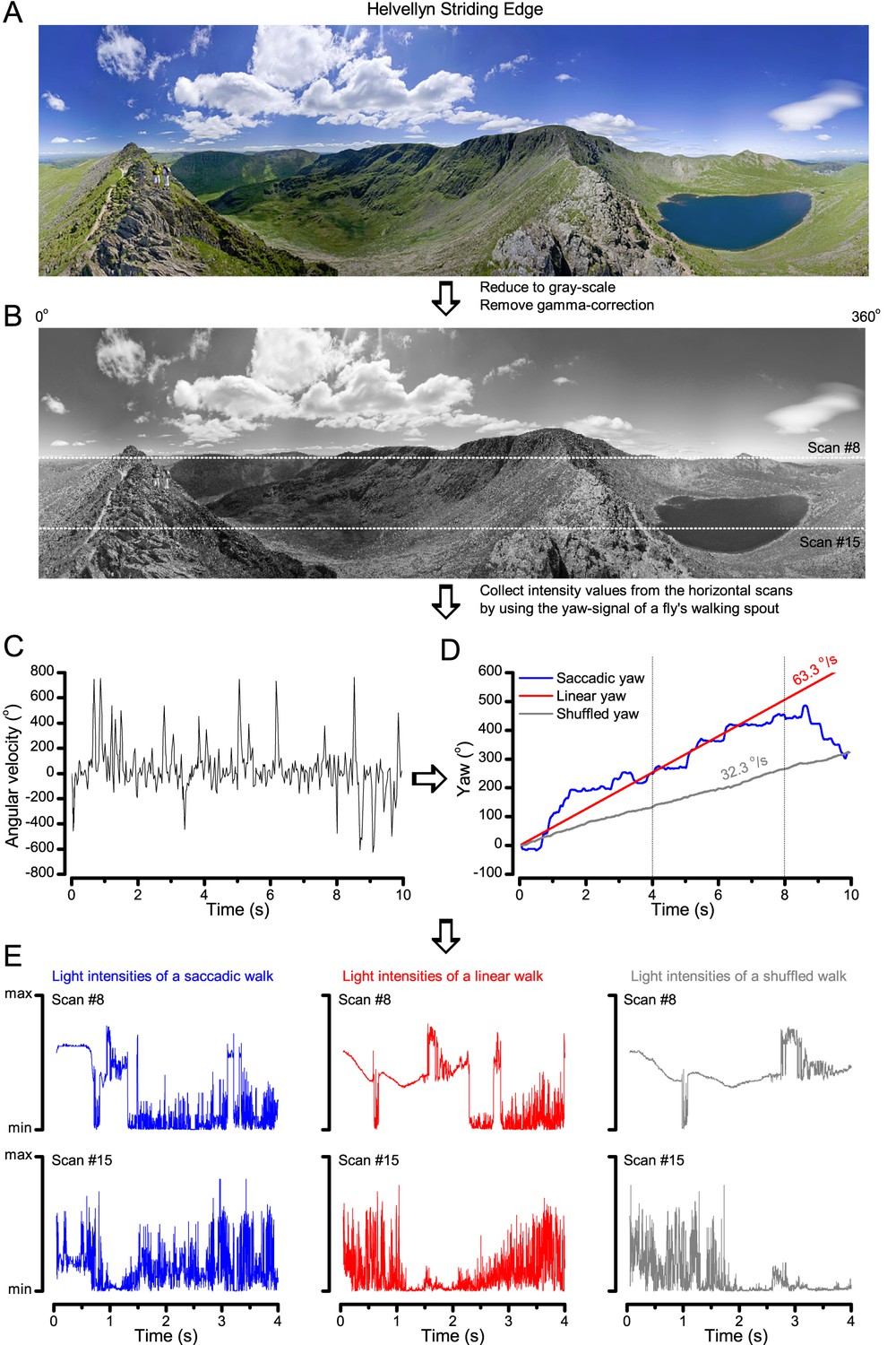
Image processing steps.
(A) 360o panoramic natural images were downloaded from the internet. (B) The images were reduced to gray-scale and their gamma-correction was removed to expose their underlying intensity differences more accurately. We then used 15 evenly spaced horizontal (x-axis) line scans to sample their relative intensity values at different vertical (y-coordinate) position. The white dotted lines show two of these scan lines. (C) Angular velocities during a free fly’s walk, from (Geurten et al., 2014). (D) These velocities were translated to a yaw signal (degree values) over time (named saccadic: blue trace). Red trace shows the linear (median) yaw signal, which corresponds to a fly walking in one direction with the fixed speed of 63.3 o/s. The shuffled yaw (gray trace) is generated by randomly selecting angular velocity values from the recorded walk (in C). (E) These three different yaw signals (o). were then used to sample intensity values from the linear line scans (in B; here shown for #8 and #15) at each 1 ms time-bin, generating unique light intensity time series from the panoramic image. Here the corresponding traces are shown for the first 4 s to highlight how differences in locomotion cause large differences in temporal light stimulation (i.e. light input to photoreceptors). Video 1 shows how these three different walking (or locomotion) dynamics (saccadic, linear and shuffled) affect the image stream to the eyes, using the panoramic ‘swamp forest’ scene (Figure 6C).
Appendix 3—figure 3
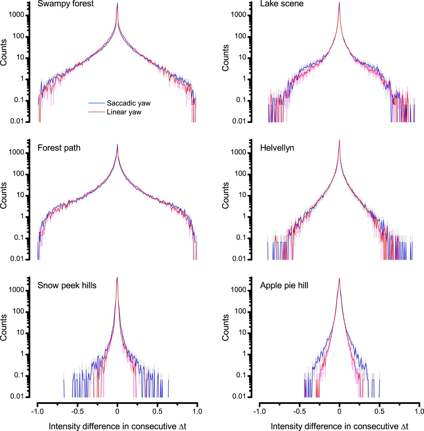
Difference histograms of the six panoramic images of natural scenes (used in this study) as scanned by saccadic (blue) and linear (red) yaw signals of the same median velocity.
Saccadic viewing increased the burstiness (Video 1) and, thus, sparseness in the difference histograms beyond that of the linear viewing. This was because saccades, proportionally, generated more large light intensity variations; seen by the extended flanks of the histograms. Conversely, fixation periods prolonged the periods of similar light intensities. Thus, the likelihood that the light intensity at one moment would be similar or the same at the next moment was increased; seen by the histograms’ higher counts for zero difference.
Appendix 3—figure 4

Photoreceptor output information rate depends on the speed and temporal structure of naturalistic stimulation (NS).
(A) Intracellular voltage responses of a blowfly (Calliphora vicina) R1-R6 to a NS sequence repeated at different playback velocities. (B) The entropy rate, RS, of photoreceptor responses increases with the playback velocity until saturation, whereas the noise entropy rate, RN, remains virtually unchanged (cf. photoreceptor noise power spectra in Figure 2—figure supplement 2A). This improves the photoreceptor's encoding performance. (C) Information transfer rate (Shannon, 1948; Juusola & de Polavieja, 2003) (R = RS RN) increases with playback velocity for four different NS sequence until saturation. Such dynamics resemble information maximization in Drosophila photoreceptor output by stimulus bandwidth broadening (Figure 2C). However, because Calliphora R1-R6s generate quicker responses than Drosophila R1-R6s, their information transfer saturates at considerably higher stimulus frequencies (Juusola et al., 1994; Juusola and Hardie, 2001b; Juusola and Hardie, 2001a; Gonzalez-Bellido et al., 2011; Song et al., 2012; Song and Juusola, 2014), suggesting superior encoding performance at high saccadic velocities. (A–C) Data is from (Juusola and de Polavieja, 2003) (Figure 5). (D) Drosophila R1-R6 output shows relative scale-invariance to NS pattern speed. NS was repeated at different playback velocities and the corresponding intracellular responses of a R1-R6 are shown above. Responses to four NS velocities are highlighted (yellow: 1 kHz, 10 s window; cyan: 3 kHz, ∼3.3 s window; magenta: 10 kHz, 1 s window; gray: 30 kHz, ∼0.3 s window). (E) The time-normalized shapes of R1-R6 output emphasize similar aspects in NS, regardless of the used playback velocity (here from 0.5 to 30 kHz). R1-R6s integrate voltage responses of a similar size for the same NS pattern, much irrespective of its speed. Mean ± SD shown, n = 7 traces. (D–E) Data is from (Zheng et al., 2009) (Figure 4).
Appendix 4—figure 1
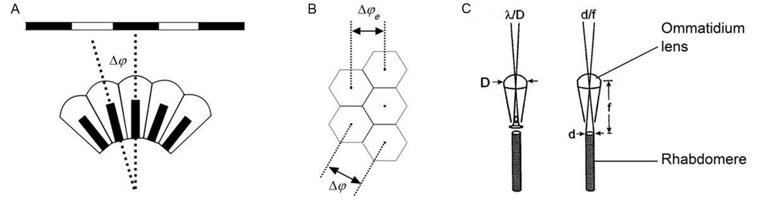
Classic theories of compound eye optics.
(A) It is assumed that the minimum angle a compound eye can resolve is its interommatidial angle, ∆φ. (B) The effective interommatidial angle of an eye with a hexagonal layout, ∆φe, is smaller than its actual interommatidial angle, ∆φ. Equation A4.1 gives their geometrical relation. (C) Light diffraction at the ommatidial lens and the rhabdomere tip strongly affects the optical quality of the image pixel that a photoreceptor samples. D = ommatidial lens diameter; d = rhabdomere tip diameter; f = focal length; λ = wavelength. Redrawn from (Land, 1997).
Appendix 4—figure 2
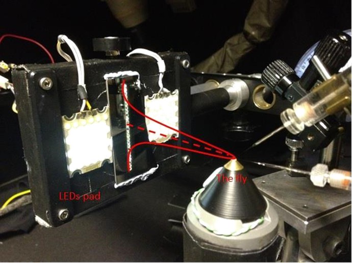
25 light-point stimulus array.
Each tested dark-adapted photoreceptor’s receptive field (red Gaussian) was assessed by measuring its intracellular responses to successive flashes from 25 light-points. In light-adaptation experiments, two 39-LED pads, (on both sides of the vertical stimulus array) provided background illumination. The intact fly was fixed inside the conical holder, which was placed upon a close-looped Peltier-element system, providing accurate temperature control (at 19°C). The rig was attached on a black anti-vibration table, inside a black-painted Faraday cage, to reduce noise and light scatter.
Appendix 4—figure 3
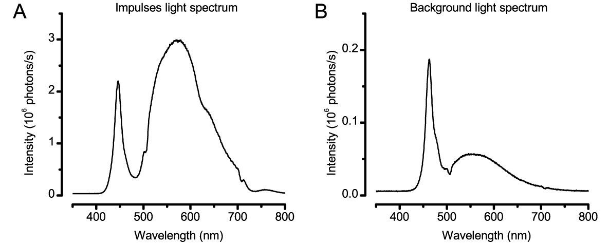
Spectral properties of the light stimuli.
(A) Typical spectral density of the light impulses delivered by the 25-point array. Note the spectra has two prominent peaks, named Peak1 (~450 nm) and Peak2 (~570 nm). (B) Spectral density of a single LED on the two Lamina pads, which were used to provide ambient background illumination during light-adaptation experiments. These spectral intensities (photon counts) were measured by a spectrometer (Hamamatsu Mini C10082CAH, Japan).
Appendix 4—figure 4
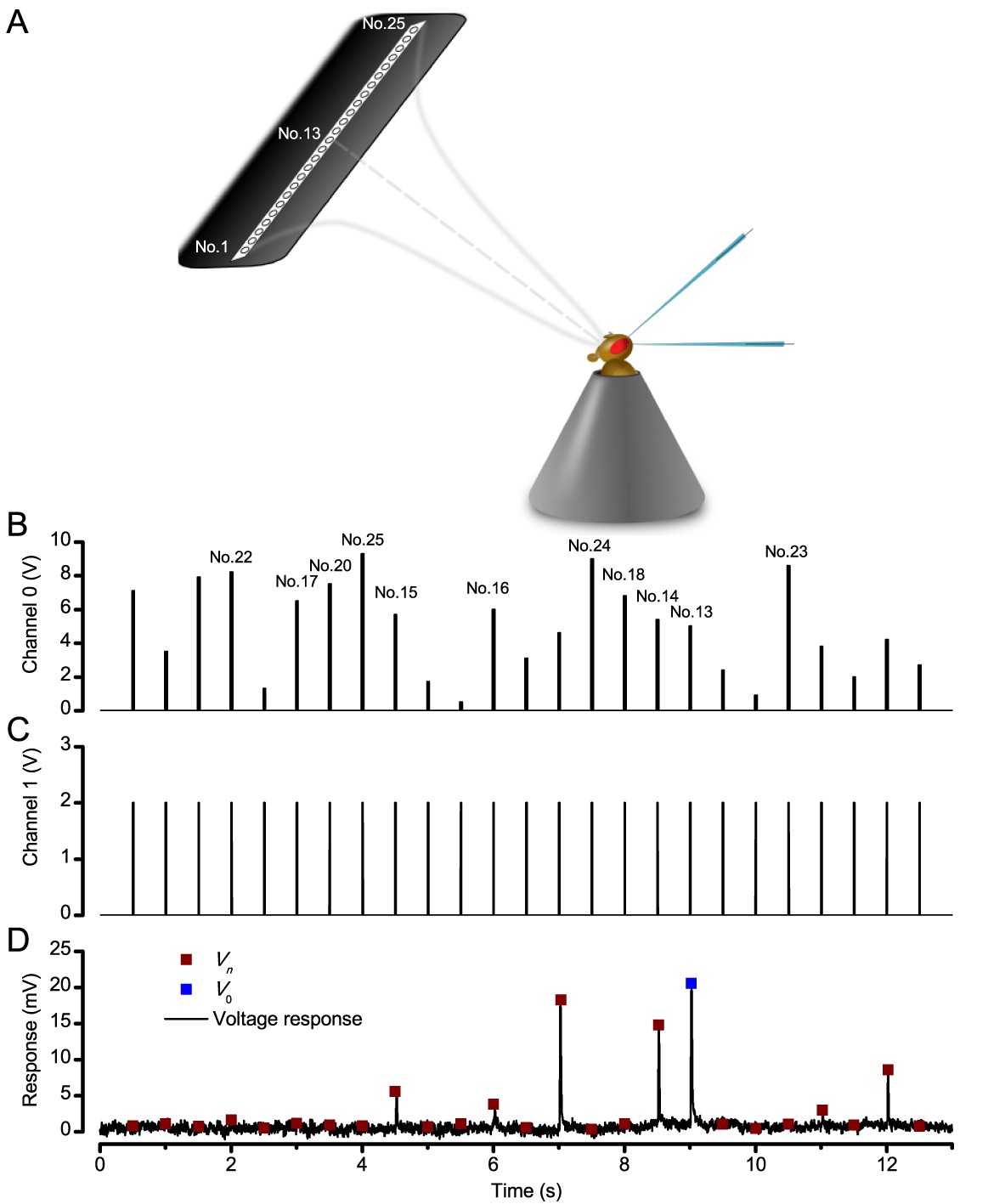
Measuring a R1-R6 photoreceptor’s receptive field with intracellular recordings.
(A) Schematic Image of how the LED stimulus array - seen as 25 light-points (light-guide-ends in a row) was centered by a Cardan arm system in respect to the studied photoreceptor and the fly eye. (B) Channel 0 input was used to select the LED (light-point) to be turned on. (C) Channel one input defined light intensity of the selected LED. A standard light impulse (flash) was produced by a 2 V input, which lasted 10 ms. (D) A photoreceptor’s intracellular voltage responses to a complete receptive field scan. These sub-saturating responses were recorded at 19°C. Amplitude Vn of each flash response was the local maxima. V0 is the amplitude of the response to a light flash at the center of the receptive field (on-axis).
Appendix 4—figure 5
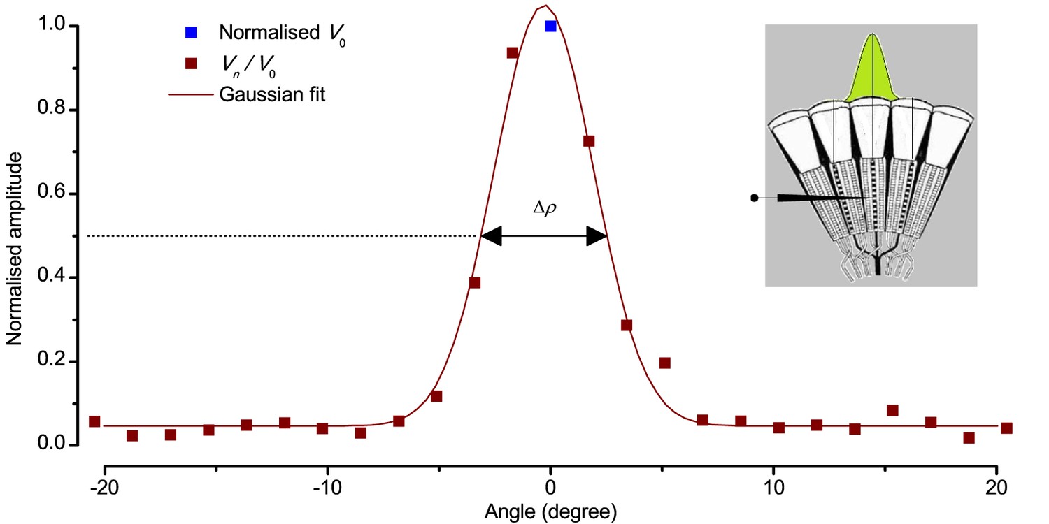
Estimating a dark-adapted Drosophila R1-R6 photoreceptor’s receptive field and its half-width.
Flash response amplitudes Vn were initially normalized to V0, the maximum response elicited by an on-axis light-point. A Gaussian curve was then fitted to these normalized values, yielding an estimate of the receptive field. Half-maximum width of this Gaussian function, ∆ρ, defined the tested photoreceptor’s acceptance angle. The schematic fly eye inset clarifies how a single photoreceptor integrates light from the world spatially through its receptive field (green area), whilst being bounded by the ommatidial lens system. For a standard measurement, each tested photoreceptor’s intracellular responses to 2–5 repetitions of pseudorandom scans (as shown in Appendix 4—figure 4) were averaged.
Appendix 4—figure 6
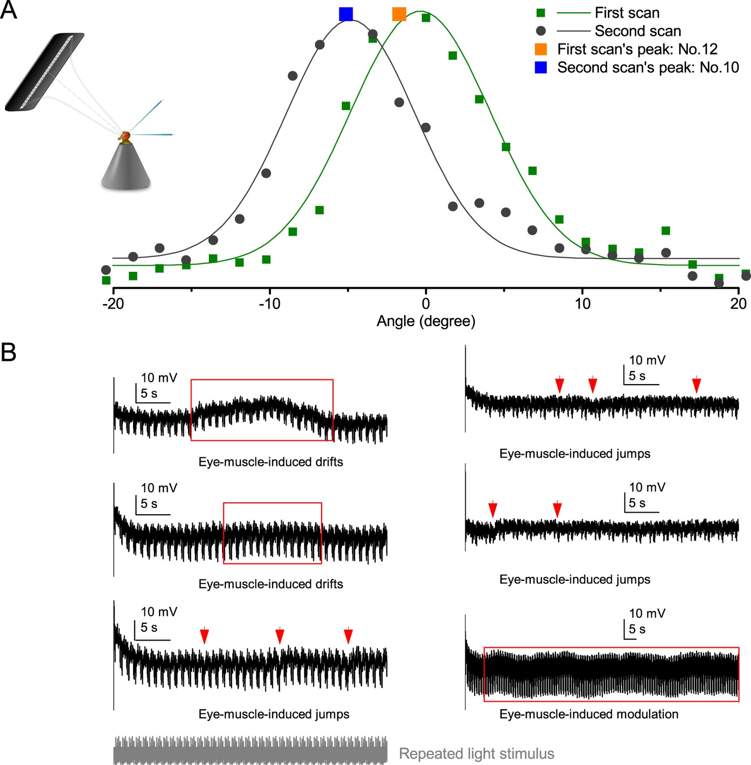
Retinal movements in the Drosophila eyes shift photoreceptors’ receptive fields, modulating their light input and hence the transduced voltage output.
(A) A R1-R6 photoreceptor’s receptive field shifted between consecutive measurements to 25 light-point stimuli. The first scan showed that the receptive field center was closest to light-point No.12; while in the second scan, the peak response was evoked by the light-point No.10. The difference between the optical axes, as indicated by the two scans, was ~3o. (B) Examples of R1-R6 photoreceptors’ intracellular responses that show slow spontaneous voltage drifts, saccades, jumps or modulation (red arrows and boxes) during repeated light intensity time series stimulation from a fixed point source. Characteristically, these perturbations do not correlate with the light stimuli but are erratically superimposed on the responses’ normal adapting trends. Because they occur in the time scale of seconds and show variable rhythmicity, they are likely caused by intrinsic eye muscle activity. Before the recordings, the light stimulus source (3o light-guide-end, as seen by the fly) was carefully positioned at the center of each tested photoreceptor’s receptive field.
Appendix 5—figure 1
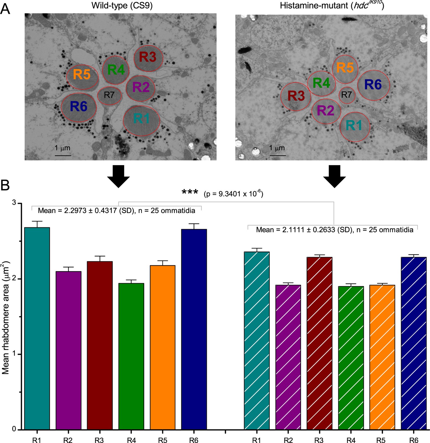
R1-R6 photoreceptors’ rhabdomere sizes differ consistently.
(A) Electron micrographs of a characteristic wild-type (left) and hdcJK910 (right) ommatidia. Each ommatidium contains the outer receptors, R1-R6, and the inner receptors, R7/R8, which can be identified by their rhabdomeres’ relative positions. Here R8s are not visible because these lie directly below R7s. Markedly, both wild-type and hdcJK910 R1-R6 photoreceptor rhabdomere sizes vary systematically. (B) The mean rhabdomere sizes measured from 25 ommatidia from 10 flies. hdcJK910 R1-R6 rhabdomere cross-sectional areas are smaller than those of the wild-type cells, but show similar proportional variations. Error bars show SEMs.
Appendix 5—figure 2
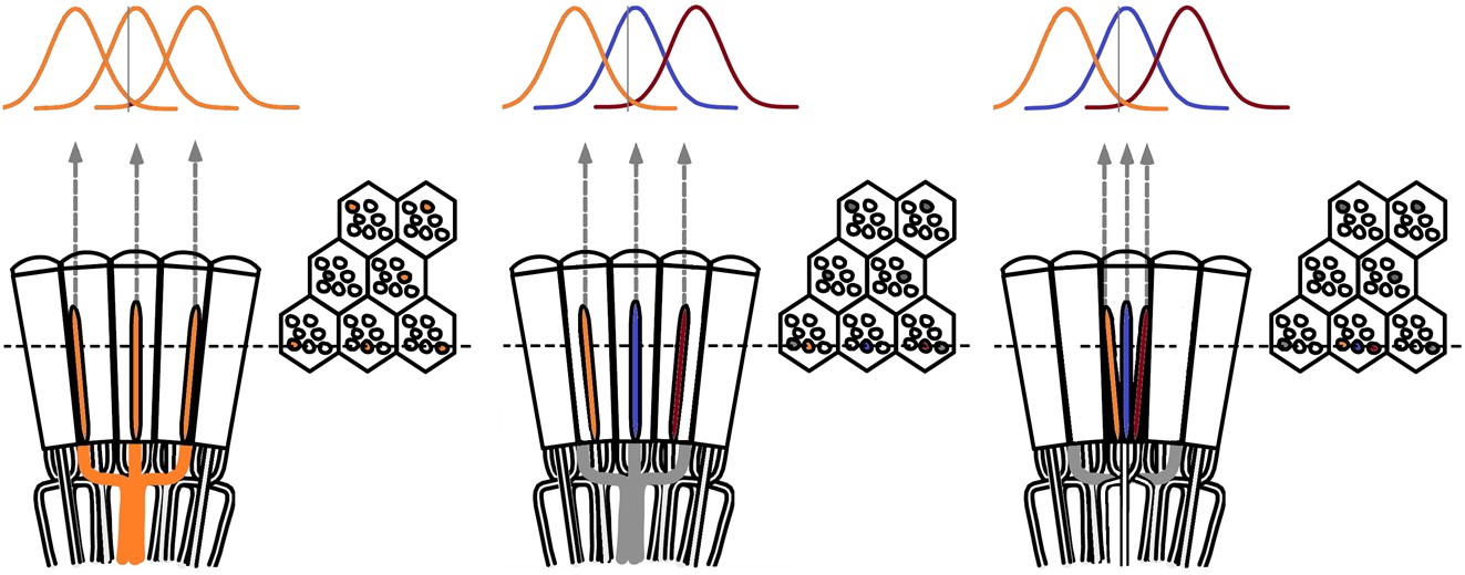
Theoretical ways to neurally improve the optical image resolution in the fly compound eyes.
Left, neural superposition with overlapping photoreceptor receptive fields. Middle, same type photoreceptors (here R2s) in the neighboring ommatidia (∆φ ~ 4.5 o) collect light from neighboring visual areas, but their receptive fields (RFs) overlap, having twice as large acceptance angles, ∆ρ ~ 9.5 o. Right, neighboring photoreceptors in the same ommatidium collect light from neighboring visual areas with their RFs overlapping. By comparing the resulting variable photoreceptor outputs from a small visual object (0.5 o vertical grey bar), neural circuitry may resolve objects finer than the inter-ommatidial angle (∆φ).
Appendix 6—figure 1
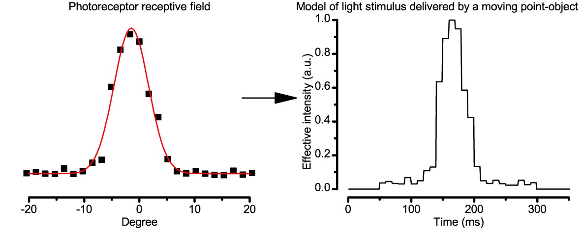
Estimating the light input from a moving object.
The effective light stimulus, which was delivered to a photoreceptor by a moving point-object, was estimated by a linear transformation of the cell’s receptive field. The width of each intensity step was calculated according to the point-object speed.
Appendix 6—figure 2
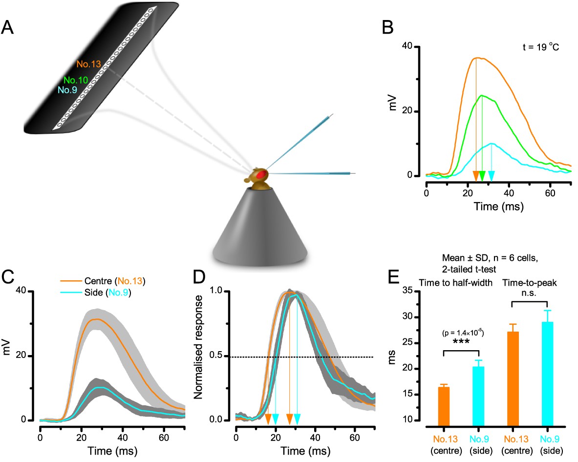
A R1-R6 photoreceptor’s sensitivity is the highest at the center of its receptive field.
(A) Schematic showing how subsaturating isoluminant light pulses were delivered at different locations within each tested photoreceptor’s receptive field. (B) The center stimulus (light-point No.13) typically evoked a response (orange trace) with the larger amplitude and faster rise-time than any stimulation at the flacks (light-points No.9 and No.10, respectively). (C) Average voltage responses of six photoreceptors to corresponding center and side stimulation. (D) Normalized responses make it clear that the responses to the center stimulus rise faster. (E) Time to the half-width response is significantly briefer (p = 1.39×10⁻⁵) with the center stimulus. However, time-to-peak of the responses to center and side light-points shows more variability between individual cells (p = 0.125). Mean ± SD; two-tailed t-test; nwild-type = 6 cells.
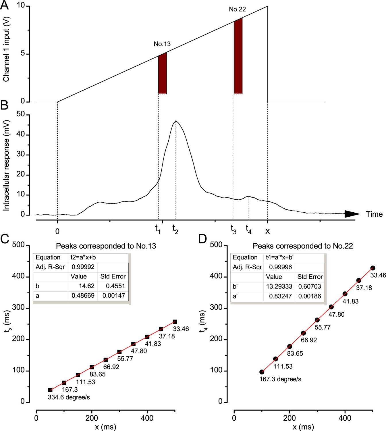
Appendix 6—figure 3
Photoreceptor response maxima lag moving objects.
(A) Channel 1 input was driven by an incremental ramp to create an image of a bright dot (point-object) moving from the No.1 light-point to the No.25 (front-to-back). Similar decremental ramps were used to produce back-to-front motion. (B) Intracellular responses of Calliphora photoreceptors to a moving point-object showed two response peaks: a large peak at t2, which corresponded to the moment it travelled pass the cell’s optical axis at t1, and a smaller peak at t4 caused by the exceptional brightness of light-point No.22, which was turn on at t3. x was the object’s travelling time. (C) An example of the linear correlation between t2 and x. Below each data point is its corresponding stimulus (dot) velocity. (D) An example of the linear correlation between t4 and x. Again, the corresponding dot velocities are shown.
Appendix 6—figure 4
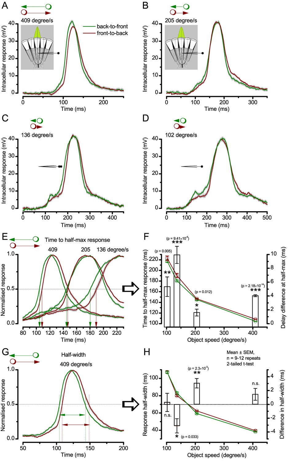
Photoreceptor output’s time-to-peak is insensitive to object motion direction but its waveforms rise and decay faster to back-to-front motion.
Examples of intracellular voltage responses of the same dark-adapted Drosophila photoreceptor to a bright dot (point-object), which crosses its receptive field in back-to-front (green) or front-to-back (brown) directions (Mean ± SEM). The insets show a schematic of the compound eye structure, with the green Gaussian representing a R1-R6’s receptive field. (A–D) Voltage responses to 409, 205, 136 and 102 °/s object speeds, respectively, plotted over the whole duration of the corresponding stimuli. (E) Whilst the similarly timed respective response peaks showed no clear directional preference, the response waveforms, nevertheless, systematically rose and decayed earlier to back-to-front (green) than to front-to-back motion (brown), irrespective of the object speed. (F) The response rise-time (measured by time to half-maximal response), decreased with increasing object motion but it was always less to corresponding back-to-front (green) than front-to-back (brown) motion. This delay difference (white bars) was significant for all the tested object speeds and varied between 2 and 10 ms (mean ± SEM, 0.01 ≤ p ≤ 2.18 x 10⁻¹⁴, 9 ≤ n ≤ 12 trials, two-tailed t-test). (G) Because the response rise and decay times changed in unity, the resulting response half-widths to corresponding back-to-front and front-to-back object motion were largely similar. (H) Accordingly, the response half-width decreased with increasing object motion, but showed only small (<4 ms) inconsistent differences (bars) between the corresponding back-to-front and front-to-back object speeds. These results are consistent with the fast light-induced photoreceptor contractions, which move their receptive fields in front-to-back direction, as observed directly in high-speed video recordings in vivo (Appendix 7).
Appendix 6—figure 5
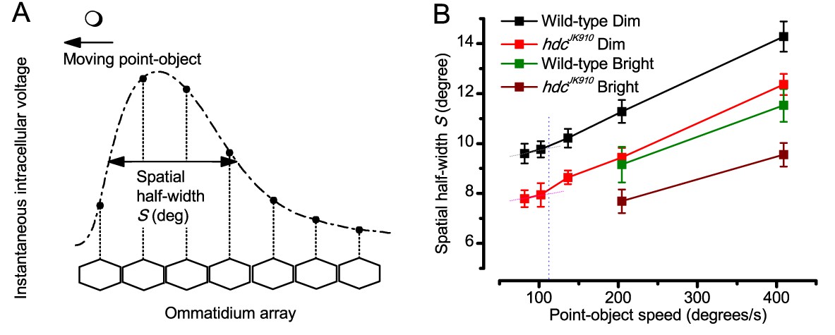
Object motion blur according to the classic theory, applied to the neural images in the Drosophila eye as it was thought to affect them in the past.
(A) Hypothetical spatial pattern of an instantaneous voltage response at an ommatidial array produced by a moving point-object. Figure redrawn from (Srinivasan and Bernard, 1975). (B) Spatial half-width of neural image of a moving point-object as a function of its speed in Dim and Bright conditions. For all the tested speeds, Shdc were significantly smaller than Swild-type (p = 0.0036–0.049, t-test), except for 205°/s in Bright condition, where the statistical test yielded p=0.137. S was calculated using data at 19°C. Mean ± SEM, nwild-type = 4–15, nhdc = 3–16, two-tailed student test.
Appendix 6—figure 6
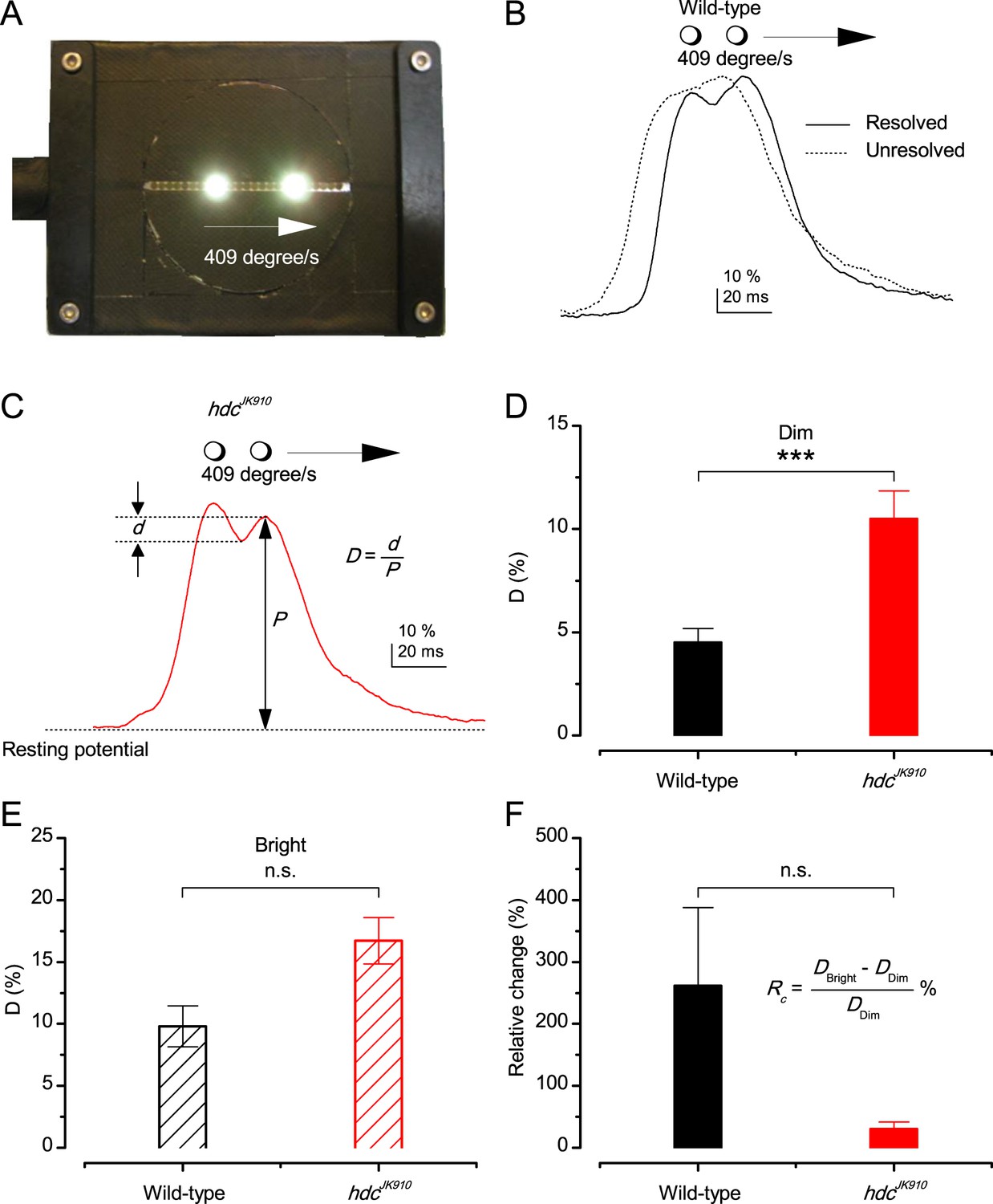
Resolving two moving point-objects.
(A) Two light-points (bright dots) moving together were presented in the tested photoreceptor’s receptive field at 19°C. The dots were 6.8° apart and travelled at 409°/s in the front-to-back direction. For clarity, neutral density filters and the LEDs pads used for background illumination are not shown in this picture. (B) In Dim, 12 out of 18 wild-type photoreceptors could resolve them, showing the response waveform depicted by the continuous line, with the larger trailing peak. While six other could not distinguish the two objects; showing the waveform of by the dotted line. In Bright, 5 out of 6 examined wild-type photoreceptors resolved the two dots. (C) Response waveform of hdcJK910 R1-R6s exhibited two distinct peaks, with the leading one was the larger. In Dim, 15 out of 16 tested mutant photoreceptors could resolve the two objects and 14 of them displayed this waveform. In Bright, all of 8 recorded hdcJK910 photoreceptor responses resolved the objects. D-values were calculated from the amplitude of the smaller peak and the dip in between. (D) In Dim, D-values of hdcJK910 R1-R6 responses were significantly larger than their wild-type counterpart. Dwild-type = 4.51 ± 0.67%, Dhdc = 10.5 ± 1.35%, p = 0.00075, t-test, nwild-type = 12, nhdc = 15. (E) In Bright, the difference of D-values of the two photoreceptor groups was statistical insignificant. Dwild-type = 9.81 ± 1.65%, Dhdc = 16.71 ± 1.86%, p = 0.117, t-test, nwild-type = 5, nhdc = 8. (F). ) Changing from Dim to Bright condition, D-values of wild-type photoreceptors appeared to exhibit larger changes than those of mutant photoreceptors. However, the difference was not statistically significant due to the large cell-to-cell variation. RC wild-type = 262 ± 126%, RC hdc = 31 ± 11%, p = 0.164, nwild-type = 4, nhdc = 7. (D–F) Mean ± SEM, two-tailed student test.
Appendix 6—figure 7
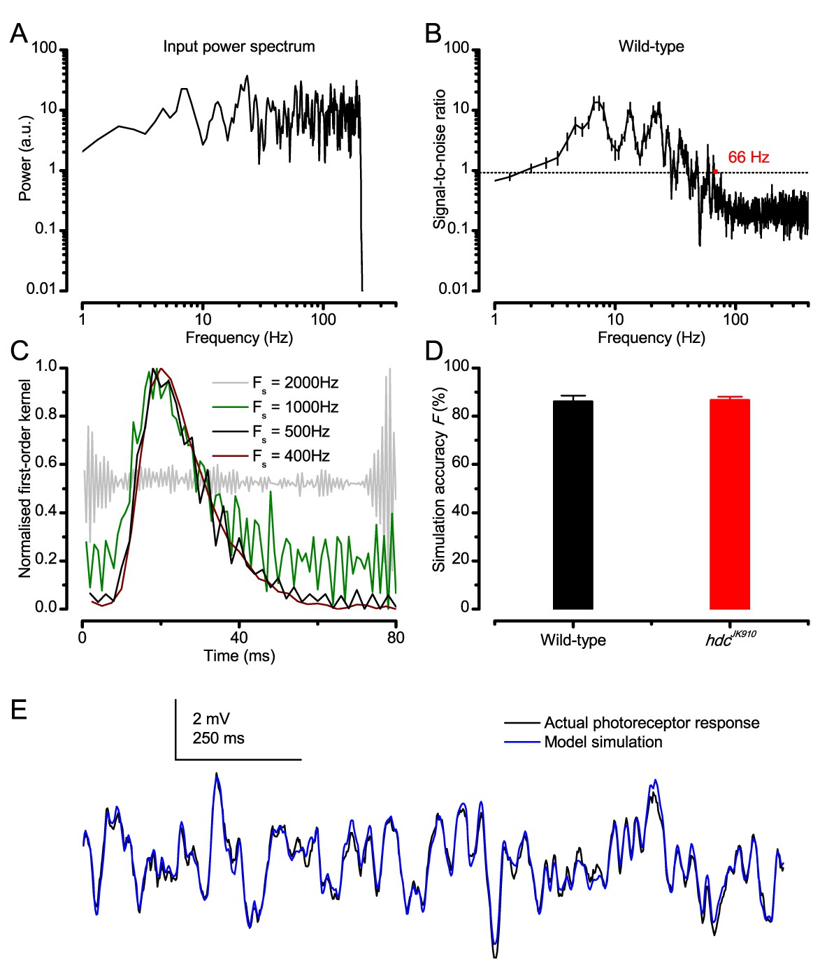
Predicting responses to Gaussian white noise (GWN).
(A) GWN light stimulus power spectrum with 200 Hz cut-off frequency. (B) Signal-to-noise ratio (SNR) of a wild-type R1-R6 photoreceptor’s voltage response at 19°C. Here, because the mean stimulus intensity was kept well within the subsaturating range (100-times lower than in the experiments of the main paper), having 200 Hz bandwidth, SNRmax of the photoreceptor output was ~ 20 (consistent with high-quality recordings for this specific stimulus condition) (Juusola and Hardie, 2001a). Noise power exceeded signal power at around 66 Hz. hdcJK910 R1-R6 outputs exhibited similar characteristics (data not shown for clarity). (C) Examples of kernels computed at different sampling rates from the same raw data. (D) Accuracy of GWN response simulation by Volterra series models for wild-type and hdcJK910 R1-R6s. Fwild-type = 86 ± 2.5%, Fhdc = 86.6 ± 1.6%. (E) Simulations of Drosophila R1-R6 responses to GWN stimuli matched the actual data closely. (B, D) Mean ± SEM, nwild-type = 9, nhdc = 8.
Appendix 6—figure 8

Prediction accuracy of the Volterra series photoreceptor models to moving point-objects varies considerably.
(A) Two examples of model simulations, which were reasonably close to the actual intracellular recordings to the tested dot motion. (B) Two examples of simulations that clearly differed from the recordings. (C) Theoretical predictions of photoreceptor output spatial half-width, calculated from the recordings and simulations as a function of the point-object speed. Mean ± SEM, nwild-type = 9, nhdc = 8. The theoretical spatial half-widths of the simulations differ from those of the recordings. E.g. the wild-type recordings (black) predicted consistently narrower S than the corresponding simulations (blue). The predicted resolvability of the resulting neural image, or spatial half-width (S), was consistently lower for the simulations than for the recordings. (D) Crucially, Volterra series models failed to predict how well the actual photoreceptor output resolves two close objects moving together very fast (shown for 409 and 818 o/s). For the 818 o/s prediction, we used here the fastest impulse response, recorded from another cell, but even so, the model still could not resolve the two dots. Thus, the actual spatial half-width of R1-R6s, limiting Drosophila’s resolving power at high image velocities, is about half of that estimated in (C). (Note, the dynamic biophysical mechanisms causing this difference – both in light input and photoreceptor output - are explained in Appendix 8. Recordings and simulations were at 19°C.
Appendix 7—figure 1

Microscope system for high-speed video recording of light-induced photoreceptor movements.
(A) High-speed camera (Andor Zyla, UK) recorded images of deep pseudopupils in the eye of an intact living Drosophila under deep-red antidromic illumination (here 740 nm LED + 720 nm long-pass edge filter underneath the fly head). Each studied fly was immobilized inside a pipette tip. (B) A 10 ms blue-green light flash, delivered through the microscope system (orthodromically) into the left fly eye (above), was used to excite R1-R8 photoreceptors; the inset below shows R1-R7 rhabdomeres (blue) of one ommatidium just before the flash. (C) Light caused the rhabdomeres to twitch photomechanically in back-to-front direction (arrows) after 8–16 ms delay, with the photoreceptors being maximally displaced in ~ 100 ms from the stimulus onset. Invariably, this was seen as a sudden jump in the recorded rhabdomere position (red). (D) The difference in the rhabdomere position (displacement) before and after the flash, depended upon the light intensity, ranging between 0.3–1.4 µm; note a typical R1-R6 rhabdomere diameter is about 1.7 µm (Appendix 5). The frame subtraction (before and after the light flash) indicates that only the rhabdomeres that aligned directly with the blue/green light source moved (within the seven central ommatidia; yellow area), while the rest of the eye remained immobile. Accordingly, the difference image shows little ommatidial walls, as these and other immobile eye structures became mostly subtracted away. In contrast, eye muscle activity, which is every so often seen with this preparation (Appendix 4, Appendix 4—figure 6) occurs more gradually and moves all the eye structures together.
Appendix 7—figure 2
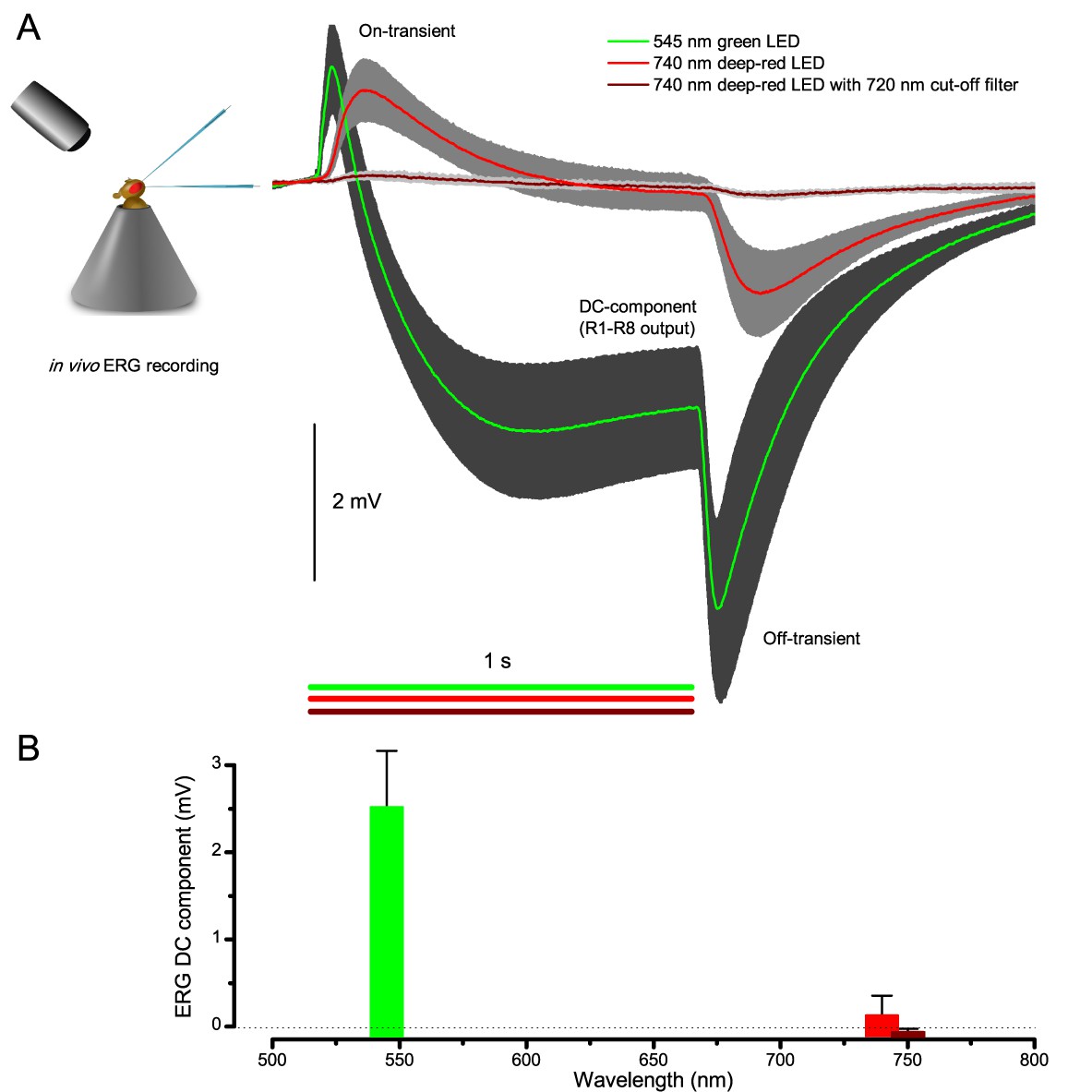
Testing R1-R8 photoreceptors sensitivity to deep-red illumination by electroretinogram (ERG) recordings.
(A) ERGs were recorded in intact Drosophila, placed inside a conical holder, to 1 s long very bright green (545 nm), red (740 nm) and deep-red (740 nm LED with 720 nm high-performance long-pass filter) pulses. A normal ERG contains a large but slow photoreceptor (DC) component and the faster on- and off-transients (Heisenberg, 1971), which signal histaminergic transmission to lamina interneurons. (B) The very small ERG response (wine) to the deep-red pulse indicated very little R1-R8 photoreceptor activation. Mean ± SD shown, n = 6–7 wild-type flies.
Appendix 7—figure 3
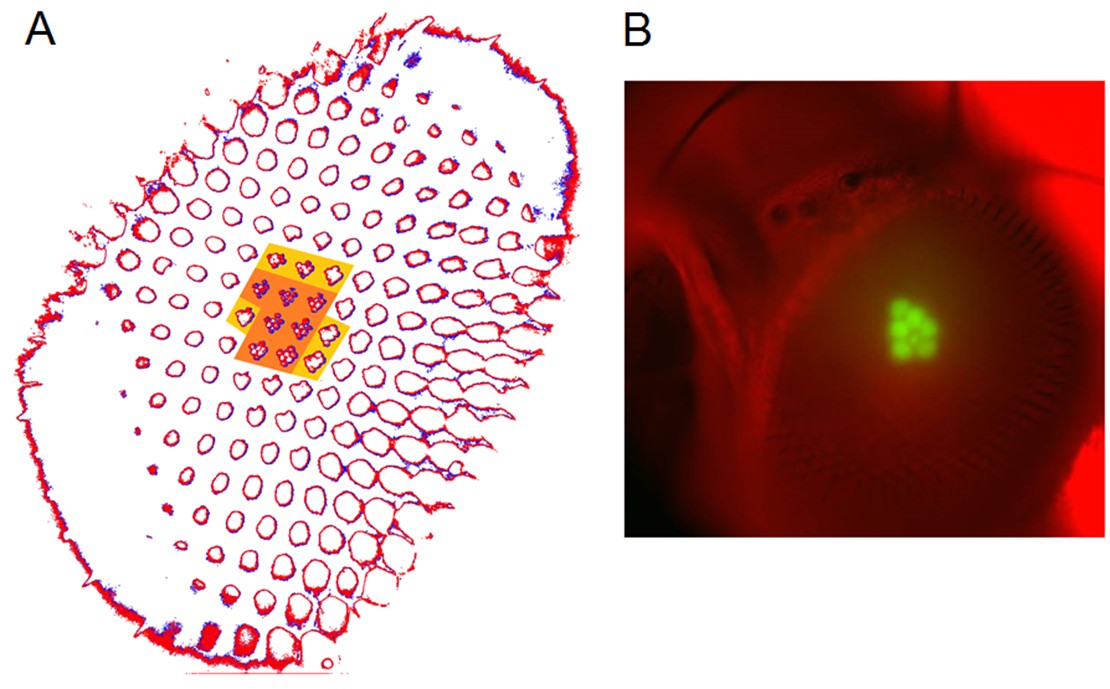
Photomechanical rhabdomere movements were localized inside those seven ommatidia that form the normal pseudopupil.
(A) High-speed video recordings in the Drosophila eye showed clear rhabdomere displacement before (marked blue) and after (marked red) a blue/green flash only within seven ommatidia (orange area). This was revealed by subtracting the corresponding frame contours. The rhabdomeres of these seven ommatidia aligned directly with the blue/green stimulus, which was carefully centered above in the microscope port (Appendix 7—figure 1). Marginal rhabdomere movements were further detected in six other neighboring ommatidia (yellow area). These results meant that only the rhabdomeres that faced the centered Orthodromic blue/green stimulus absorbed its light and contracted, while the rest of the eye reflected this stimulus and remained immobile. Note that this local rhabdomere activation pattern was restricted by the same eye design principle that causes the insect eye pseudopupil. (B) The Drosophila eye, in which photoreceptors were made to express green-fluorescence, displayed a green pseudopupil only form those seven ommatidia that directly faced the observer (and the blue light source through the microscope lenses). This happened because these ommatidia (their rhabdomeres) both absorbed the incident blue light and their GFP-molecules released green light back to the observer’s eye/camera, while the other ommatidia around reflected the blue light.
Appendix 7—figure 4
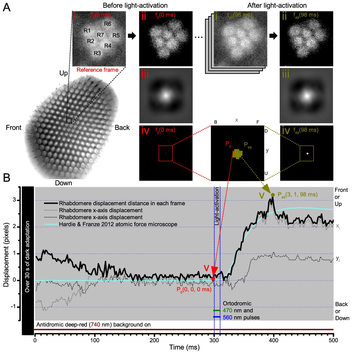
Cross-correlation image analysis to estimate photomechanical R1-R7 rhabdomere movements.
(A) Analytical steps are shown for the reference frame at time zero (f0), 2 ms before the 10 blue/green light stimulus pulse (red), and for the frame at the maximum rhabdomere displacement (f49), 98 ms after (dark yellow). High-speed camera images of rhabdomeres were recorded using 750 nm red light. (i) Image stacks were uploaded, and (ii) the median of each frame was subtracted to remove its noise background. (iii) 2D cross-correlation was calculated for each frame, and (iv) the values within 5% of their peak value were selected. (v). ) The weighted mean peak positions gave each frame’s x- and y-positions at its specific time point, and their distance, sqrt(x2+y2), the total rhabdomere displacement (in pixels) against the reference frame position. Notice that the 2D cross-correlation images have flipped x- and y-axis directions (up, U, appears down, D; front, F, appears back, (B). (B) The resulting rhabdomere displacement distance and the corresponding x- and y-positions are plotted for each frame in time at 2 ms resolution (500 frames/s), against the reference frame position, P0(0, 0, 0). A comparable (inverted) atomic force microscopy data (cyan) closely matches the rise-time dynamic of the cross-correlation rhabdomere displacement estimate, validating our analytical approach. The analysis also implies that well dark-adapted photoreceptors may respond weakly to deep-red (740 nm) light onset (black trace 0–100 ms). Note R8 rhabdomere, which lies directly below R7, likely contracts too.
Appendix 7—figure 5
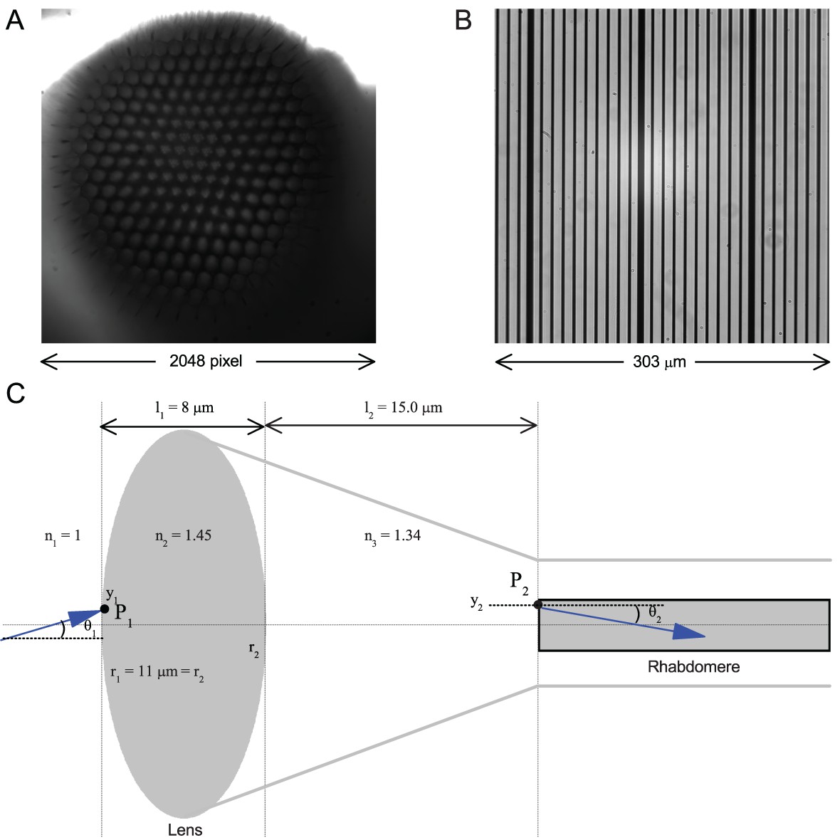
Calibrating the rhabdomere displacements in microns and their receptive field movements in degrees.
(A) A whole image of a Drosophila’s left eye, the camera chip’s full 2048 × 2,048 pixel range. (B) a high-resolution graticule placed at the same focal plane as the image (A) gives the full image size of 303 × 303 µm. Thus one pixel ~ 0.1479 µm. (C) A schematic of the main optical components in a normal Drosophila ommatidium. Its optical properties indicate that a 1 µm rhabdomere displacement shifts its receptive field by 3.56°.
Appendix 7—figure 6
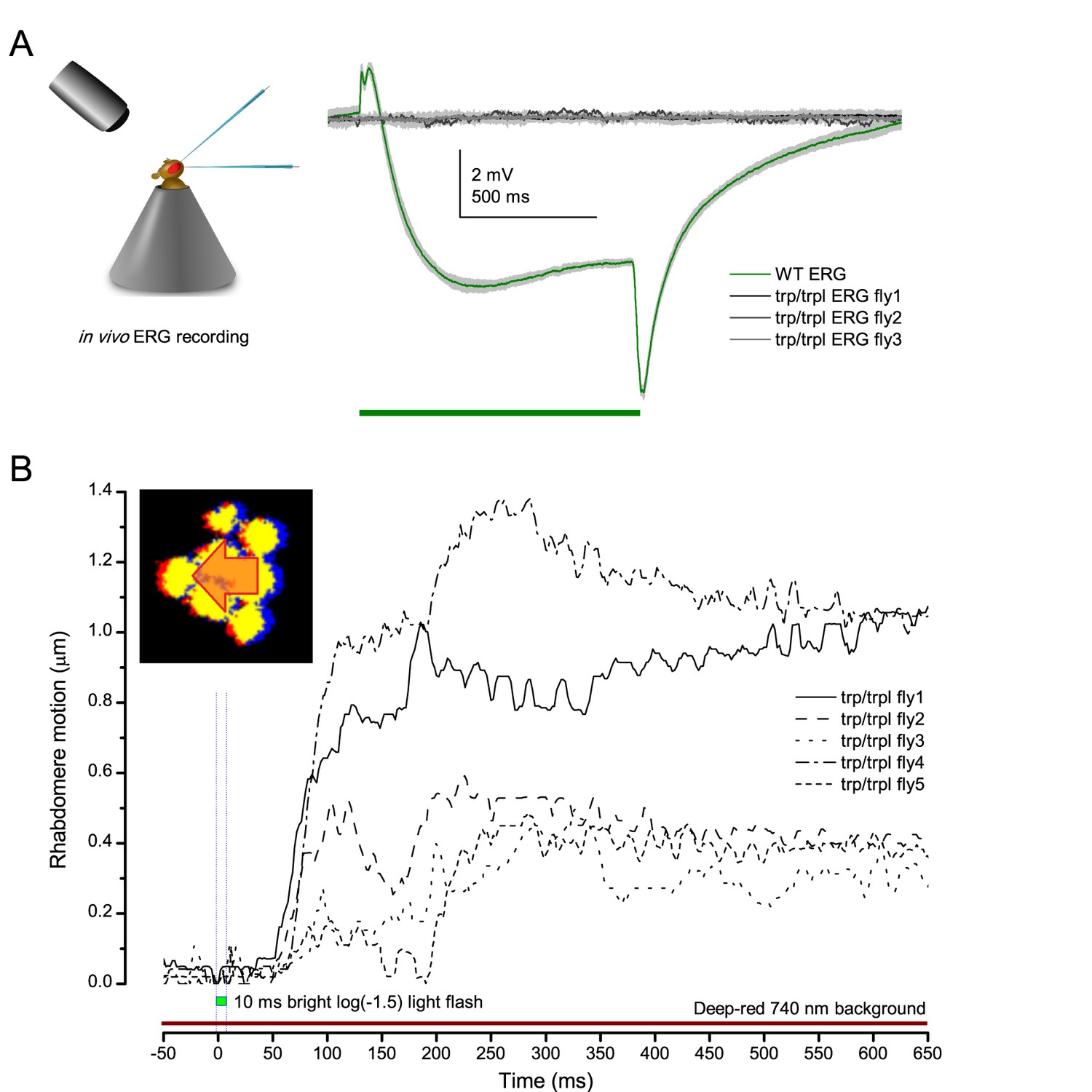
Photoreceptors of blind trp/trpl null-mutants flies show photomechanical contractions.
(A) ERGs of trpl/trpl mutants show no electrical activity indicating that these flies are profoundly blind. (B) High-speed video recordings at their rhabdomeres show light-induced lateral movements, indicating that (i) these photoreceptors contact photomechanically and (ii) these movements cannot involve eye muscle activation.
Appendix 7—figure 7
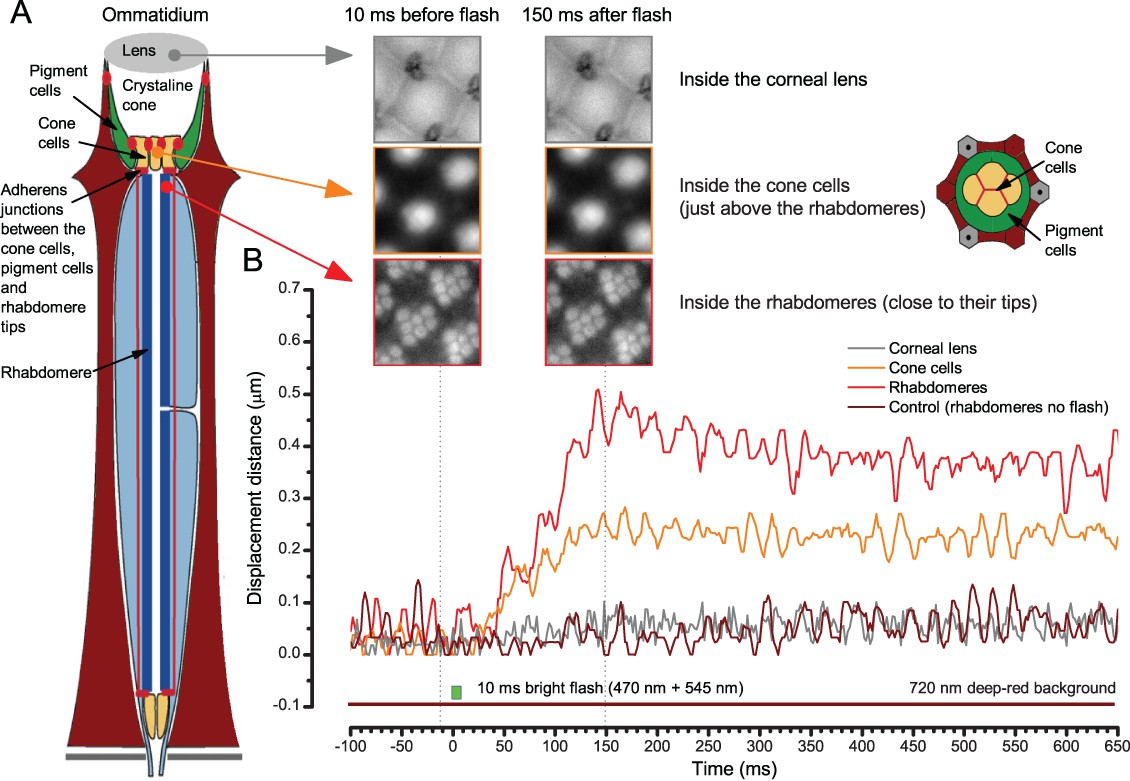
When the rhabdomeres move the ommatidium lens stays still.
(A) High-speed video recordings at different depths inside ommatidia before and after a bright light flash. (B) Cornea (ommatidium) lens and the optical structures to the narrow base of the crystal cone remained virtually immobile. Below these, the cone cells showed movement that was half of that seen in the rhabdomeres. In the schematic, red dots and lines indicate adherens junctions that link the photoreceptors to the pigment and cone cells.
Appendix 7—figure 8
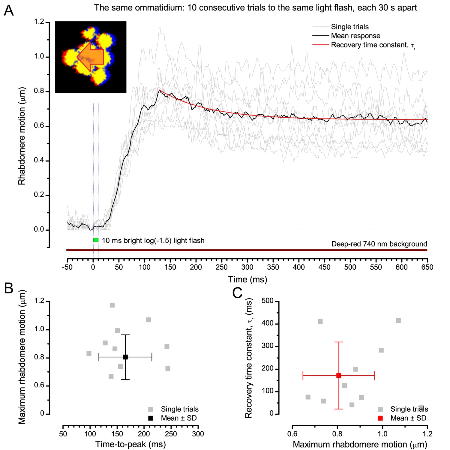
Photomechanical rhabdomere motion is robust and repeatable.
(A) Consecutive rhabdomere motions (grey thin traces) of the same ommatidium and their mean (black) to 10 stimulus repetitions (bright flash). The mean response recovery is fitted with an exponential, τr. (B) Each response maximum is shown against its time delay (time-to-peak) with the mean and SD. (C) Each response recovery time constant is plotted against its maximum with the mean and SD. Recording at t = 20°C.
Appendix 7—figure 9
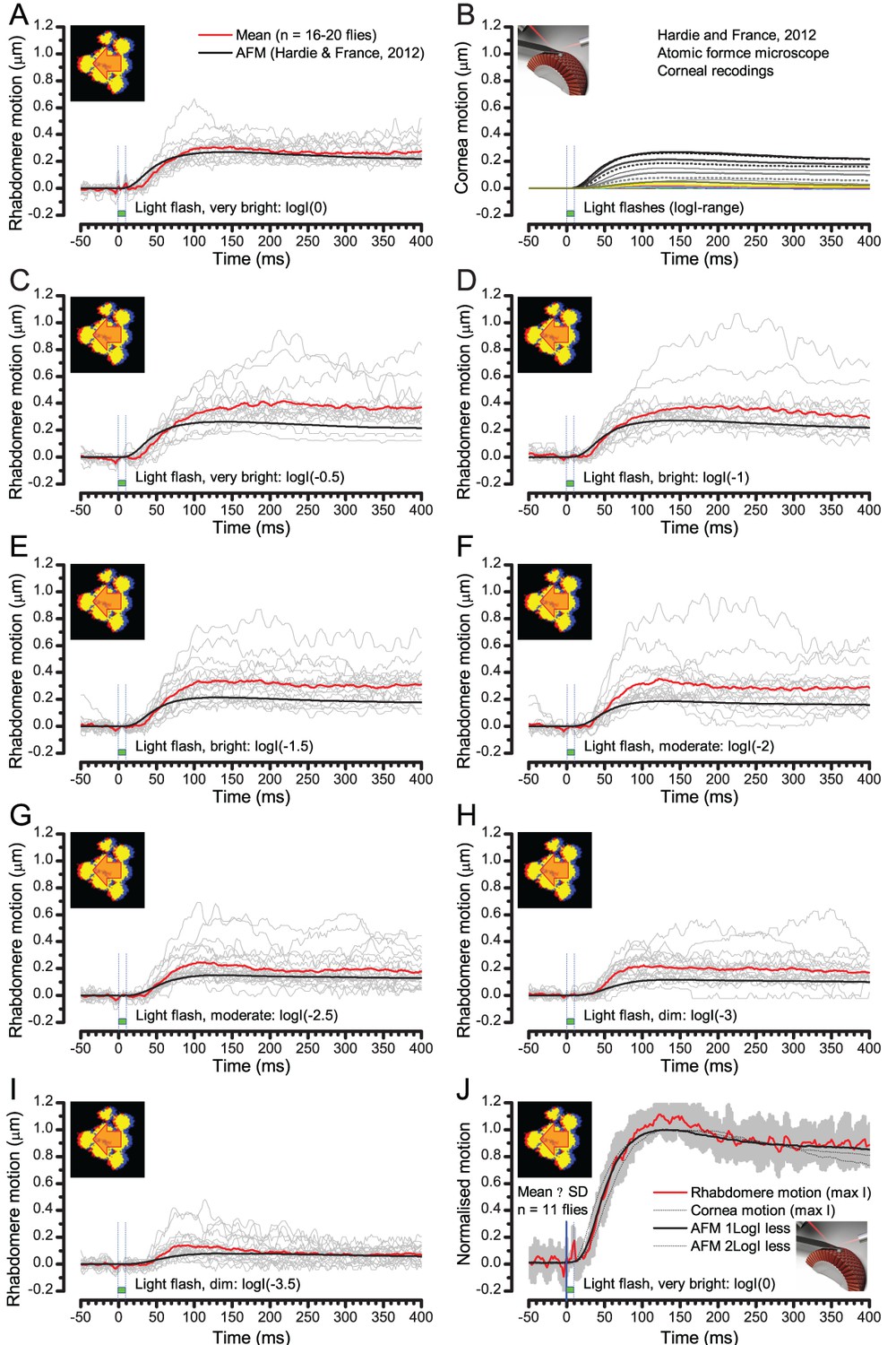
Comparing optically resolved wild-type rhabdomere movements to corresponding atomic force microscope (AFM) recordings from the corneal surface.
To ease the comparisons, the AFM data is inverted. (A) Rhabdomere motion within individual ommatidia (grey thin traces) and their mean (red) evoked by the brightest 10 ms test flash are plotted against the largest AFM recording (black) to the brightest 5 ms test flash (data from Hardie and Franze, 2012). The rhabdomere movement range is larger than what the AFM data suggests. (B) AFM recordings to a broad logarithmic light flash intensity range. (C–I Rhabdomere movements vs. AFM recordings to light flashes of broadly comparable diminishing intensities. Notice that some individual rhabdomere movement recordings show minor oscillations that could be related to recording noise or physiological activity. (J) the mean and SD of normalized rhabdomere movements to the brightest test flash are compared with the normalized AFM recordings to three different test flash intensities. All these AFM recordings fall within the SD of the given rhabdomere recordings.
Appendix 7—figure 10

Photomechanical rhabdomere contractions in dissociated ommatidia.
(A) Two frames of high-speed video footage of contracting R1-R8 photoreceptor rhabdomeres in vitro, evoked by a bright flash. The size-view imaging reveals the size and dynamics of their photomechanical lengthwise changes. (B) Characteristic maximum longitudinal rhabdomere contractions range from 0.8 to 1.7 µm. Thus, in an intact eye, during contractions the rhabdomeres would move inwards, away from the lens. This movement is likely to move the rhabdomere tips into the ommatidium lens’ focal point, narrowing the photoreceptors’ acceptance angles (see Appendix 8, Appendix 8—figure 3). Notably, many rhabdomeres also twist during these contractions, providing additional crosswise movements. See Video 2.
Appendix 7—figure 11
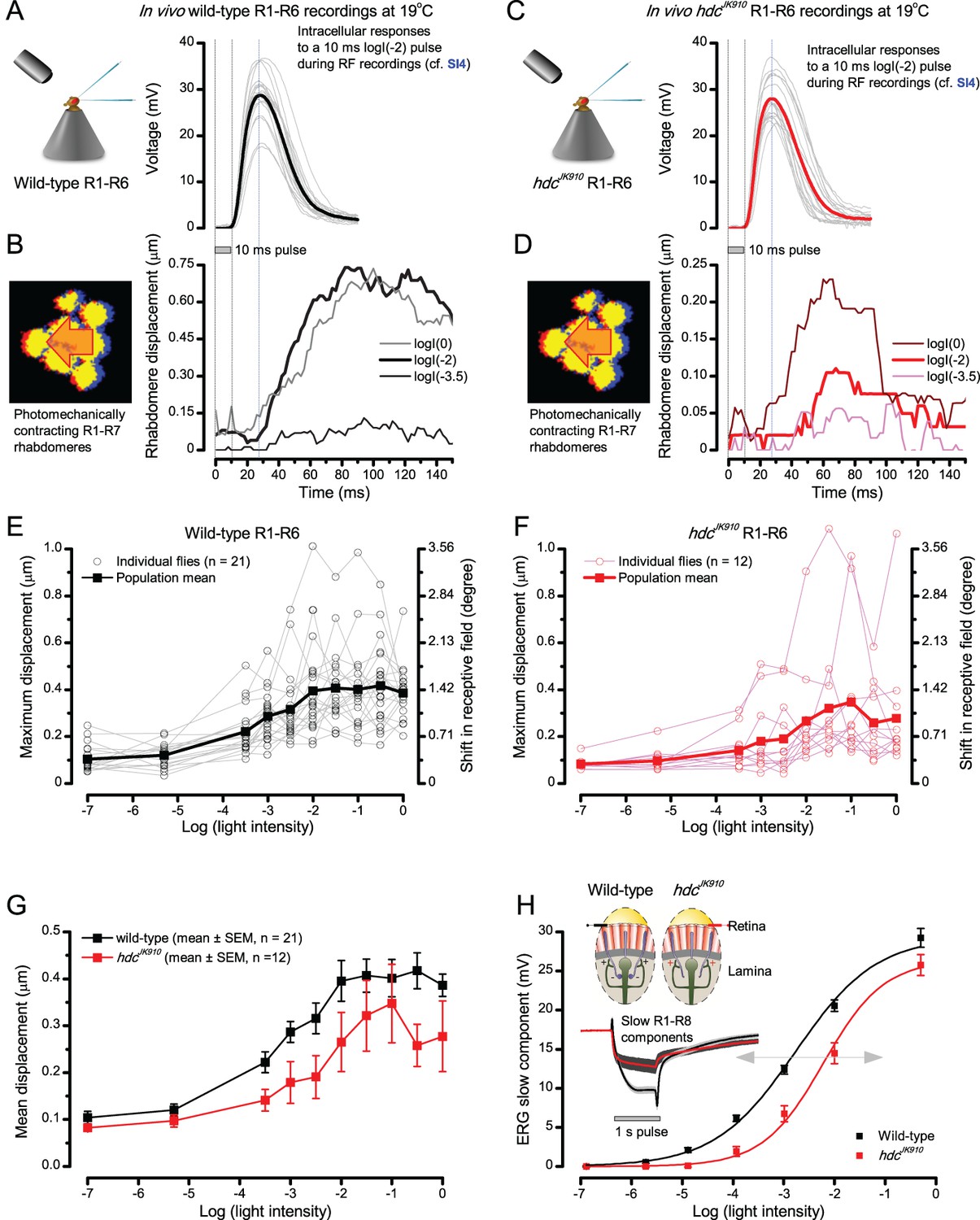
Comparing dark-adapted wild-type and hdcJK910 R1-R6s’ photomechanical rhabdomere contractions to their corresponding electrophysiological responses at 19°C.
(A) Intracellular voltage responses of dark-adapted wild-type R1-R6s to a 10 ms subsaturating light pulse, delivered at the center of their receptive field. (B) Characteristic non-averaged photomechanical rhabdomere movements (displacement in time) of a typical wild-type fly, as quantified by the cross-correlation analysis (Appendix 7—figure 4) to very dim (log(−3.5)), moderate (log(−2)) and very bright (log(0)) 10 ms light flashes. (C) Intracellular responses of dark-adapted hdcJK910 R1-R6s to a similar stimulus (as in a). (D) hdcJK910 rhabdomere movements to very dim, moderate and very bright 10 ms flashes are characteristically slightly smaller than the corresponding wild-type recordings in (B). (E) The wild-type and (F) hdcJK910 rhabdomere displacements increase with logarithmic light intensity. (G) Mean wild-type rhabdomere movement was larger than that of hdcJK910 over the tested intensity range, with the hdcJK910 photoreceptors’ apparent right-shift indicating a 10-fold reduced sensitivity. (H) This right-shift is broadly similar to these photoreceptors’ V/LogI characteristics, measured from their ERG slow components (Dau et al., 2016).
Appendix 7—figure 12
Wild-type photomechanical rhabdomere movement dynamics at different light-adaptation states.
Characteristic non-averaged photomechanical rhabdomere movements of 7 wild-type flies and their means (thick traces) to bright (logI(−1); left) or to very bright (logI(0); right) light flashes. The recordings were performed in relative darkness (>720 nm) or when the eyes were adapted for 30 s to different green (545 nm) or blue (470 nm) light intensity levels; from weak (logI(−3)) to bright (logI(−1)). (A–B) In dark-adaptation, consistent with the results in Appendix 7—figure 11, the brighter the flash, the larger and faster the evoked mean rhabdomere movements. (C–D) Prolonged blue light exposure converted virtually all Rh1-rhodopsins to their active meta-form, causing a PDA (prolonged depolarizing afterpotential). PDA increases the photoreceptors’ intracellular calcium load, cleaving PIP2 from the plasma-membrane and so keeping them in a contracted state. A very bright green flash rapidly converts some of the meta-Rh1 back to Rh1, enabling small and brief rhabdomere movements, which resemble those seen with hdcJK910 flies (Appendix 7—figure 11). (E–H) Adaptation to different green-light intensity levels did not abolish rhabdomere movements to light increments. These movements can, in fact, be larger than in the same cell’s dark-adapted state, as was seen in Fly4 and Fly6 recordings. Notice that a 1.2–1.4 µm rhabdomere displacements means ~4-5o shifts in a R1-R6 photoreceptor’s receptive field (Appendix 7—figure 4), which can be more than the average Drosophila interommatidial angle.
Appendix 8—figure 1
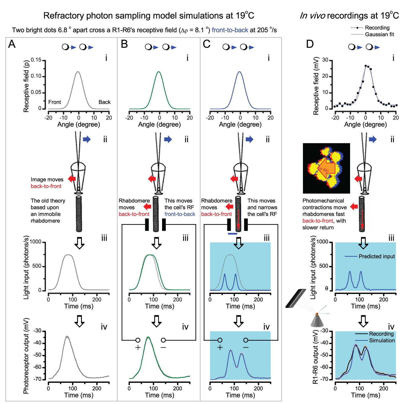
Microsaccadic sampling-hypothesis predicts R1-R6 output dynamics to fast moving bright dots.
We compare stochastic sampling model predictions of increasingly realistic light input modulation (A–C to real recordings D). In each case, the light stimulus is two fast moving bright dots (i), which cross a R1-R6’s receptive field (RF, half-width = 8.1o) front-to-back at 205 o/s. The immobile ommatidium lens focusses their light onto a rhabdomere tip (ii). But because of diffraction, their images blur (airy disk). Interestingly, however, in Drosophila, the airy disk half-width (~1.7oor ~ 0.6 µm) is smaller than the rhabdomere diameter (~1.7 µm; Appendix 5). The dynamic light input falling upon the rhabdomere (iii) is then estimated by convolving the two dot intensities with the cell’s receptive field over time (i). This light input is sampled stochastically by 30,000 microvilli, in which quantum bumps integrate the dynamic voltage response (iv). (A) In the simulations, where the rhabdomere is stationary during the dots flyby (corresponding to the classic theory (Srinivasan and Bernard, 1975; Juusola and French, 1997), ii), their light fuses together (iii). This is because the simulated photoreceptor’s RF half-width (8.1o) is wider than the distance between the dots (6.8o). Accordingly, the photoreceptor output (iv) cannot distinguish the dots. (B) Next, we include the light-induced fast back-to-front rhabdomere movement in the model (ii; as measured in the high-speed video recordings in Appendix 7, Appendix 7—figure 1), but keep the cell’s RF shape the same. The resulting RF movement makes the light input rise and decay slightly later than in the previous case (iii; cf. the green and dotted grey (A) traces), but still cannot separate the two dots. The resulting photoreceptor output (iv) shows a single peak, which is slightly broader than the output from the immobile cell in (A). (C) In the full model, as the contracting rhabdomere jumps away from the focal point (ii), the light input both moves with the cell’s RF and dynamically narrows it from 8.1o to 4.0o. These processes differentiate the light input (from the dots) into two separate intensity spikes over time (iii), which the photoreceptor output can clearly separate in two distinctive peaks (iv). (D) In vivo intracellular photoreceptor recordings from a wild-type R1-R6 to the two moving dot stimulus show comparable dynamics to the full model’s prediction. In the simulation, the same cell’s RF (i) was moved and narrowed dynamically (ii-iii) according to our hypothesis in (C). This close correspondence, which occurred even without the additional response accentuation from the synaptic feedbacks (Appendix 6), implies that Drosophila photoreceptors’ RFs must move and narrow with their photomechanical rhabdomere contractions. Appendix 8—figure 3 proposes four mechanisms to narrow RF.
Appendix 8—figure 2
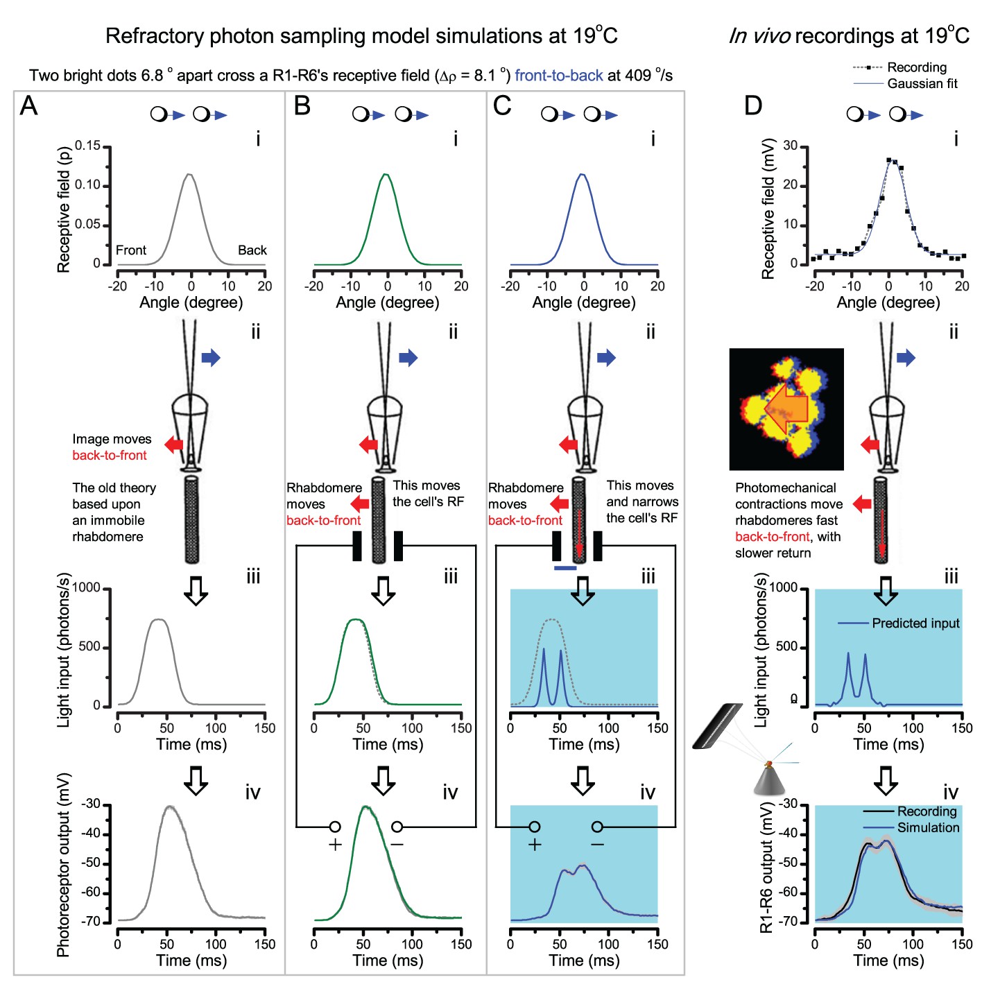
The hypothesis predicts R1-R6 output to double-fast moving point-objects.
All the parameters of the simulations are fixed to the experimentally measured values, similar to Appendix 8—figure 1. The stimulus is the same two bright dots, but this time, they cross the cell’s receptive field (RF) double-fast, 409o/s (i). (A) Again, if the rhabdomere remains stationary during their flyby (corresponding to the classic theory, ii), their light fuses (iii), and the photoreceptor output cannot distinguish the dots (iv). (B) By including the light-induced back-to-front rhabdomere movement (ii) but with the same RF shape, the light input broadens slightly (iii), but cannot separate the two dots. Consequently, the photoreceptor output (iv) shows a slightly narrower single peak than in the previous case in (A). (C) If, however, the rhabdomere contraction (away from the lens’ focal point, ii) moves the RF and actively narrows it (from 8.8o to 4.9o), the light input from the dots is transformed into two intensity spikes (iii), which R1-R6 output separates into two peaks (iv). (D) Corresponding intracellular R1-R6 recordings show comparable dynamics to the full model (C). These and other simulations and recordings, which all show good correspondence, establish that photoreceptors’ RFs must move and narrow dynamically during light stimulation.
Appendix 8—figure 3
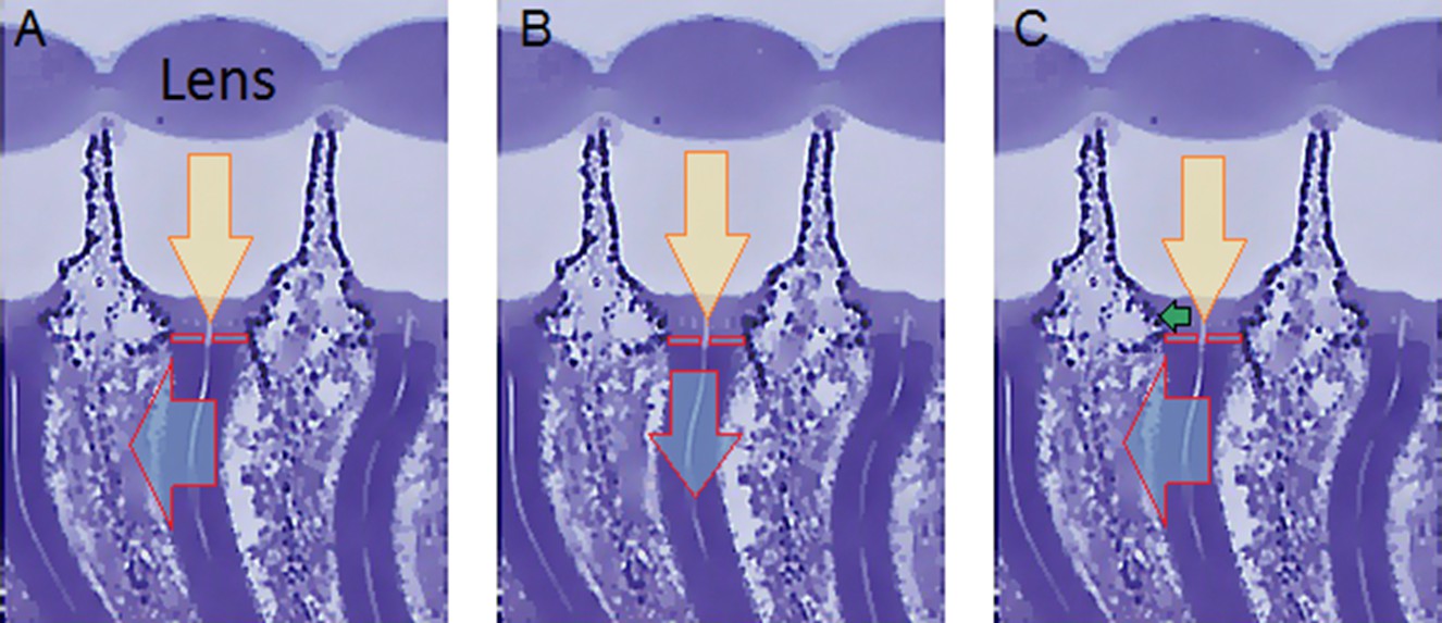
How ommatidium dimensions change during light-induced photoreceptor contractions.
The three images show the same transverse section of three Drosophila ommatidia, with their rhabdomeres appearing as six darker curvy strips. The rhabdomeres contract (cyan arrow) to light (yellow arrow, as focused by the lens), moving both (A) horizontally (back-to-front) and (B) vertically (down arrow), see Appendix 7. Because the rhabdomeres are connected to the surrounding structures by adherence junctions (Tepass and Harris, 2007) (red boxes highlight the transition areas), their contraction induces (C) moving and possibly narrowing of the aperture (green horizontal arrow) formed by the cone and pigment cells, which are directly above the rhabdomeres (lighter blue areas). Ultimately, the curvature of the lens and focal distance might also change slightly. Image modified from (Gonzalez-Bellido et al., 2011).
Appendix 8—figure 4

The new hypothesis predicts and the recordings show that R1-R6 output rises and decays earlier to a back-to-front moving bright dot than to a front-to-back moving dot of equal velocity.
(A) A classic model with (i) a symmetrical receptive field and (ii) an immobile rhabdomere leads to identical (iii) light inputs and virtually identical (iv) photoreceptor outputs (minute differences result from stochastic photon sampling), respectively, for the dots moving in the opposite directions. (B) A model with (ii) a moving rhabdomere generates both dynamic (iii) light input and (iv) photoreceptor output, which rise and decay earlier for the back-to-front moving dot (red traces) than the front-to-back moving dot (blue traces). (C) Our full model with rhabdomere contraction dynamics that move and narrow its receptive field. This makes the light input and photoreceptor output rise and decay faster than in the other two models, with the back-to-front waveforms leading the front-to-back counterparts. (D) The intracellular responses of a R1-R6 photoreceptor to the given two dot stimuli, as recorded in vivo, show similar dynamics to the full model in (C) with its back-to-front signals (red) leading the front-to-back signals (blue).
Appendix 8—figure 5
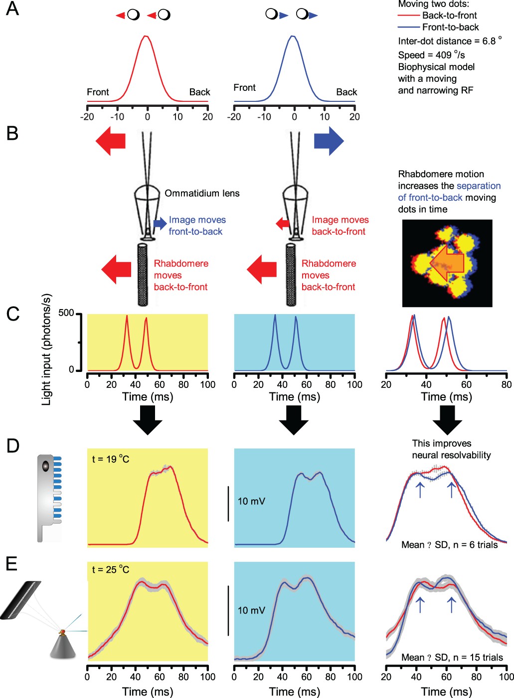
Fast rhabdomere movements are predicted to improve the resolvability of fast front-to-back moving objects the most.
(A) Two bright dots, 6.8o apart, cross a photoreceptor’s receptive field (RF; ∆ρstart = 8.1o) either in back-to-front (red, left) or front-to-back (blue, middle) at 409 o/s (i). (B) The new photoreceptor model translated the light-induced back-to-front rhabdomere motion into concurrent RF narrowing (∆ρend = 4.0o) and front-to-back movement (as reversed by the ommatidium lens). (C) Consequently, the light input from the dots was transformed into two intensity spikes. These spikes were further apart in time for the front-to-back moving dots and for the opposing stimuli. (D) The two peaks in in the corresponding model-predicted R1-R6 output (blue) for front-to-back moving dots (highlighted by arrows) indicated that the dots were neurally detectable. In contrast, the predicted R1-R6 output for back-to-front moving dots (red) failed to separate these two point-objects at 19°C. (E) An example of intracellular recordings from one R1-R6 photoreceptor to the same two stimuli at 25°C. This cell’s voltage responses also resolved the front-to-back moving dots better than their back-to-front moving counterparts. These and other comparable simulations and recordings suggest that microsaccadic rhabdomere movements improve the neural resolution (and representation) of fast moving visual objects.
Appendix 8—figure 6
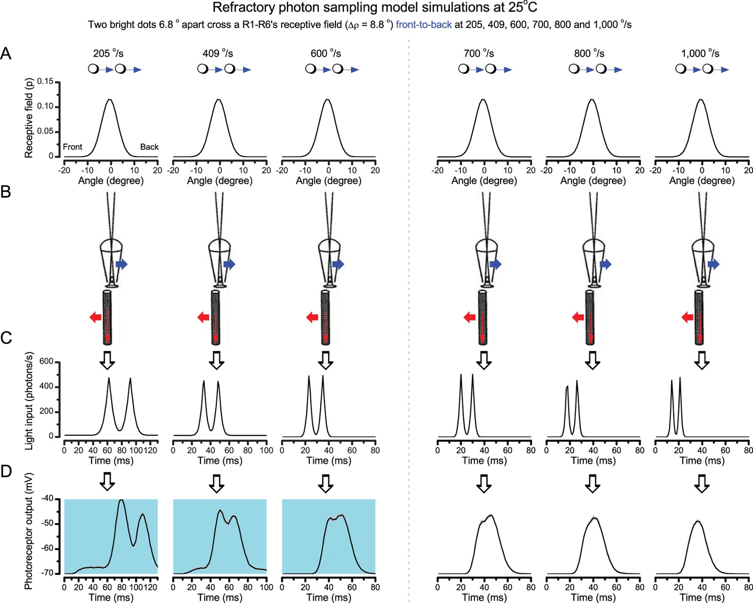
The hypothesis predicts that at the preferred temperature (25°C) Drosophila R1-R6 photoreceptors can distinguish two bright dots 6.8 o apart travelling together at ~ 600 o/s.
(A) The starting and ending receptive field size (RF; ∆ρstart = 8.1o; ∆ρend = 4.0o) in all the simulation was the same. (B) in every case, the rhabdomere contracted, moving and narrowing the RF. (C) This translated light input into two clear sharp peaks. (D) Photoreceptor output separated the dots as two peaks at velocities until above 600 o/s (left, cyan background), indicating that they were neurally resolvable. At 700 o/s or higher speeds (right), the dots were not resolved as the outputs had only a single peak. Mean ± SD shown, n = 6 repeated stochastic simulations to each stimulus.
Appendix 8—figure 7
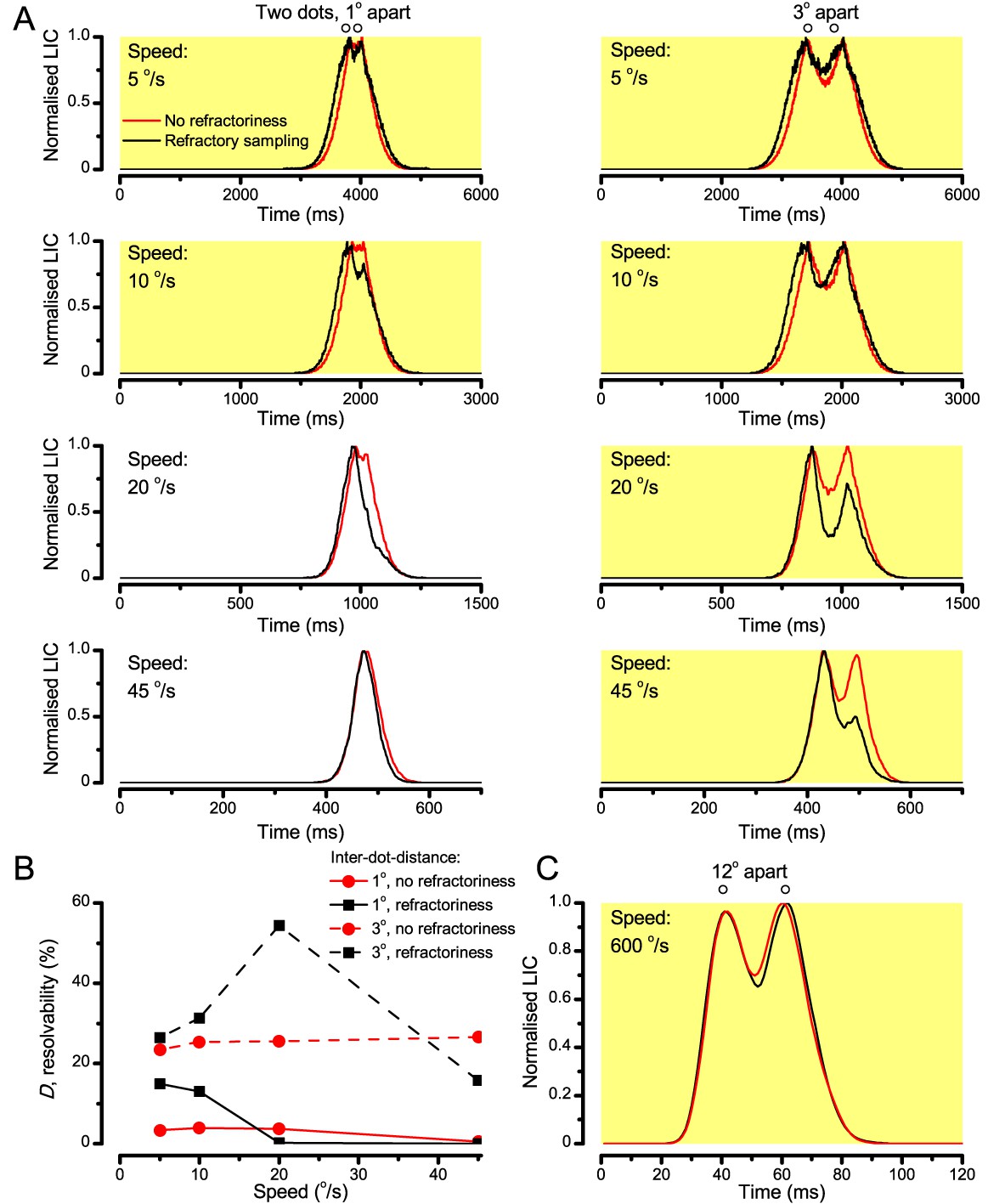
Refractory sampling enhances neural resolution for different aspects of hyperacute images.
(A) Examples of simulated macroscopic light-induced current responses (normalized LICs) of two different photoreceptor models. Both models have 30,000 microvilli. In the first model (red), every photon causes a quantum bump; hence, its photon sampling has no refractoriness. In the second model (black), photon sampling is refractory. Both models are stimulated with the same moving two bright dots, with their actual light inputs being first modulated by photomechanical rhabdomere contractions (following the microsaccadic sampling hypothesis). Based on the tests with different velocities and inter-dot-distances, refractoriness consistently causes a phase lead in LIC responses. (B) Refractoriness improves response resolution for hyperacute stimuli (inter-dot-distance <4.5o) at slow velocities (≤20 o/s). The resolvability, D, of the recordings and simulations, was determined by Raleigh criterion (cf. Figure 7C). (C) An example of how refractoriness can enhance response resolution for larger stimulus separations at high saccadic velocities. The difference from the lower peak to the trough is larger in the black trace (refractory photon sampling) than in the red trace (complete photon sampling).
Appendix 8—figure 8
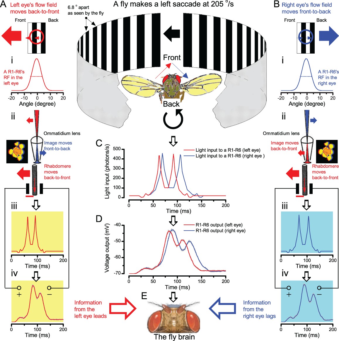
During a left saccade, signals from the left-eye lead the signals from the right-eye.
Because incoming light, in both the left and right eyes, contracts their rhabdomeres in the back-to-front direction, photoreceptors can transmit information about the field rotation or the fly’s orientation changes to the brain. Specifically, the output from the eye towards which the fly turns phase leads, and thus neurally signals rotation direction. Here we illustrate the underlying mechanism by using a brief 205 o/s left saccade (in a world of 6.8o black-and-white gratings), as an example. (A) During the left saccade, the flow field facing the left eye moves back-to-front (red arrow) across its photoreceptors’ receptive fields (i). The image of the moving flow field is inverted by the ommatidium lens, and so moves front-to-back (blue arrow) while being sampled by the rhabdomere (ii). Light contracts the rhabdomeres in back-to-front direction (red arrow). With the projected image and the photon-sampler (rhabdomere) moving against each other, the light input from two bright bars (iii) becomes narrowed and accelerated. Accordingly, photoreceptor output shows two prominent peaks, in which distance to each other is compacted in time (iv). (B) During the left saccade, the flow field facing the right eye moves front-to-back (blue arrow) across its photoreceptors’ receptive fields (i). Again, the ommatidium lens inverts the image, which now moves back-to-front (red arrow) over the rhabdomere (ii), which contracts in the same direction (red arrow). With the projected image and the rhabdomere moving together, the light input from two bright bars (iii) excites the photoreceptor longer, in which output shows two prominent peaks elongated in time (iv). (C) The light input to the left eye photoreceptors (red trace) rise and decay faster than the corresponding light input (blue trace) to the right eye photoreceptors. (D) R1-R6 output in the left eye (red trace) is faster and briefer than the photoreceptor output (blue trace) in the right eye. (E) Consequently, by correlating the outputs from the left and right eye photoreceptors in time, the fly brain can obtain information about the directional changes in the visual space, in respect to its head orientation.
Appendix 9—figure 1
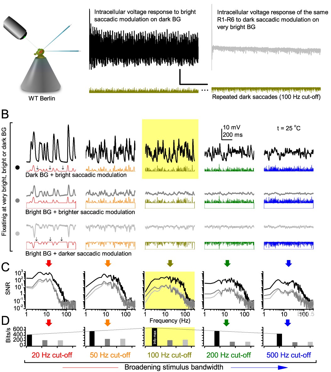
Optimal saccadic viewing strategy for maximizing R1-R6 photoreceptors’ information capture requires fixating on darker image features.
(A) Intracellular responses of a R1-R6 to repeated saccadic bright (left) and dark (right) bursts. (B) Output to bright saccadic bursts was always more vigorous when mixed with dark fixation periods (BG, above) than with bright periods (middle), irrespective of the stimulus frequency distribution. When the same R1-R6s were fixated (light-adapted) on a bright background (below), they still responded well to dark saccadic bursts (of the inverse waveforms), but the amplitude range of these responses was less than to bright bursts (above, dark BG). (C) Corresponding R1-R6 output signal-to-noise ratios were the highest for the bright-saccadic-burst/dark-fixation-period stimuli (black traces). Signal-to-noise ratios were lower but alike for the brighter saccades with bright fixation periods (grey) and the dark saccades with bright fixation periods (light grey). (D) Information transfer rates confirmed the global maximum for 100 Hz bright saccade-like bursts with dark fixations (black bars; cf. Figure 2C). Whilst bright fixation periods reduced information (with more microvilli becoming refractory), the bit rates for bright (grey) and dark (light grey) saccadic modulation, of equal but opposite contrasts, were similar.
Appendix 9—figure 2
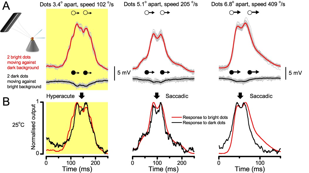
Comparing R1-R6s’ intracellular responses to hyperacute or saccadic bright or dark moving dots.
(A) Mean (thick traces) and individual responses (thin) of three individual R1-R6s to two bright (red, above) or dark (black, below) dots (of different inter-dot-distances and speeds), crossing the cells’ receptive fields in front-to-back direction. Responses to the hyperacute dots (3.4o inter-dot-distance) are shown left; responses to the saccadic speed stimuli in the middle (205 o/s) and right (409 o/s). In all cases, these outputs resolved the two dots, but predictably the responses were always smaller to the dark dots at the bright background than to the bright dots at the dark background (as more microvilli should remain refractory when adapting to bright background). (B) The normalized and sign-inverted R1-R6 outputs to dark dots were similar to their normalized outputs to bright dots, with both showing equally good Raleigh-resolvability (cf. Figure 7C). Naturally, as the Drosophila eye samples light information from each point in space by eight photoreceptors (due to neural superposition) and balances this estimate with those of the neighboring lamina cartridges, its perception/resolvability of hyperacute and saccadic image motion is improved further.
Videos
Video 1
Using a Drosophila’s saccadic walk to extrapolate light input to its photoreceptors from natural scenes
A published recording of a fly’s saccadic walk (Geurten et al., 2014) was used to sample light intensity values from 360o panoramic images of natural scenes. We collected three types of light stimuli, resulting from: (a) saccadic, (b) median (linear) and (c) shuffled velocities of the walk.
Video 2
Drosophila R1-R8s in dissociated ommatidia contract photomechanically
Wild-type and trp/trpl-mutant R1-R8 photoreceptors contract photomechanically to light flashes. The panels show: top, a sideview of ex vivo wild-type R1-R8 photoreceptors of a single dissociated ommatidium contracting to 1 ms bright light flash; bottom left, R1-R8 of a trp/trpl null-mutant, which express normal phototransduction reactants but lack completely their light-gated ion channels, contracting to a similar flash. Notably, trp/trpl photoreceptors cannot generate electrical responses to light, with their eyes showing no ERG signal (Appendix 7). Nonetheless, trp/trpl-mutant photoreceptors contract photomechanically (but require ~5 min dark-adaptation between flashes to restore their contractility). These observations are consistent with the hypothesis of the light-induced phosphatidylinositol 4,5-bisphosphate (PIP2) cleaving from the microvillar photoreceptor plasma membrane causing the rhabdomere contractions (Hardie and Franze, 2012). Video playback slowed down and down-sampled to reveal the contractions, which otherwise would be too fast to see with a naked eye. Each video clip is repeated three times with a running timer giving the time course of the contractions. Notice that the longitudinal contractions reduce the photoreceptor length. Thus, in an intact compound eye, the rhabdomeres would move inwards, away from the lens, likely narrowing their receptive fields (see Appendix 7, Appendix 7—figure 10 and Appendix 8, Appendix 8—figure 3).
Video 3
Drosophila R1-R8 photoreceptors contract photomechanically in vivo, moving back-to-front inside each observed ommatidium
We utilized the optical cornea-neutralization technique with antidromic deep-red (740 or 785 nm peak) illumination to observe deep pseudopupils (photoreceptor rhabdomeres that align with the observer’s viewing axis) in the Drosophila eye. High-speed video captures fast rhabdomere movements to bright orthodromic blue-green flashes (470 + 535 nm peaks). The panels show: left, R1-R7 photoreceptor rhabdomere tips moving rapidly back-to-front and returning slower to each 10 ms flash, delivered repeatedly every second; right, the cross-correlated horizontal (blue) and vertical (red) components as the time series of this movement. Grey vertical lines indicate each flash. The rhabdomere movement is caused by the photomechanical photoreceptor contractions (not by muscle activity). These in vivo movements are large, here 1.7 µm from dark-adapted rest-state; causing up to five degree transient shift in the R1-R6 photoreceptors receptive fields (Appendix 7). Note average diameter of R1-R6 rhabdomeres is 1.7 µm (Appendix 5). The high-speed video rate was 500 frames/s. Video playback slowed down and down-sampled to reveal the contractions, which otherwise would be too fast to see with a naked eye.
Video 4
While R1-R8s contract, the lens above is immobile but a cone-cell aperture, connected to the rhabdomere tips by adherens junctions, moves half as much as the rhabdomeres
We used a z-axis micromanipulator to shift and reposition Drosophila in piezo-steps vertically underneath the microscope. This allowed the focused image, as projected on the camera, to scan through each studied ommatidium, providing exact depth readings in µm. We then recorded any structural movements inside the ommatidia to light flashes at different depths; from the corneal lens down to the narrow base, where the cone and pigment cells form an intersection between the crystalline cone and the rhabdomere. The left panels show: up, ommatidium lens; middle, basal cone/pigment cell layer; down, R1-R7 photoreceptor rhabdomeres tips during and after flash stimulation. The right panels show the cross-correlation time series of these high-speed videos: up, the corneal lens and the upper ommatidium structures were essentially immobile), and normally remained so throughout the recordings; Middle, cone cells that connect to the rhabdomere tips with adherens junctions (Tepass and Harris, 2007) showed clear light-induced movements; down, R1-R7 rhabdomeres moved half as much as the cone cells above. The high-speed video rate was 500 frames/s. Video playback slowed down and down-sampled to reveal the contractions, which otherwise would be too fast to see with a naked eye.
Tables
Appendix 3—table 1
The used six panoramic high-resolution digital images of natural scenes were downloaded from:
https://doi.org/10.7554/eLife.26117.050| https://commons.wikimedia.org/wiki/File:Swampy_forest_panorama.jpg |
| https://commons.wikimedia.org/wiki/File:2014-08-29_11_51_08_Full_360_degree_panorama_from_the_fire_tower_on_Apple_Pie_Hill_in_Wharton_State_Forest,_Tabernacle_Township,_New_Jersey.jpg |
| https://en.wikipedia.org/wiki/File:Helvellyn_Striding_Edge_360_Panorama,_Lake_District_-_June_09.jpg |
| https://commons.wikimedia.org/wiki/File:Schleienl%C3%B6cher_Hard_360%C2%B0_Panorama.jpg https://farm3.staticflickr.com/2820/9296652749_7c502de9e7_o.jpg |
| http://www.bodenstab.org/panorama/images/Green%20Valley/panorama.jpg |
Appendix 4—table 1
Light flash peak wavelengths and intensities delivered by each of the 25 light-points in the stimulus array
The given light intensities were measured at the light source by Hamamatsu Mini C10082CAH spectrometer, before 100-fold neutral density filtering. Thus, these values are estimated to be 102-3-times higher than the corresponding effective photon rates at the level of R1-R6 sampling (see Appendix 2—figure 3). Accordingly at the optical axis, the center LED (No.13), with the neutral density filter on it, evoked subsaturating (~20–35 mV) responses from Drosophila R1-R6 photoreceptors (Appendix 4—figure 4).
Light- Point | Peak1 wavelength (nm) | Peak1 intensity (106 photons/s) | Peak2 wavelength (nm) | Peak2 intensity (106 photons/s) |
|---|---|---|---|---|
| No.1 | 448 | 2.720 | 571 | 2.805 |
| No.2 | 452 | 1.790 | 570 | 2.818 |
| No.3 | 448 | 2.618 | 565 | 2.900 |
| No.4 | 451 | 1.840 | 576 | 3.020 |
| No.5 | 451 | 2.570 | 575 | 3.710 |
| No.6 | 451 | 2.214 | 572 | 3.640 |
| No.7 | 452 | 1.430 | 575 | 2.020 |
| No.8 | 446 | 2.203 | 570 | 2.990 |
| No.9 | 453 | 1.465 | 571 | 2.350 |
| No.10 | 451 | 3.300 | 578 | 5.100 |
| No.11 | 453 | 1.877 | 575 | 3.080 |
| No.12 | 455 | 1.763 | 575 | 3.020 |
| No.13 | 451 | 2.334 | 575 | 3.440 |
| No.14 | 451 | 2.009 | 576 | 2.634 |
| No.15 | 454 | 2.400 | 568 | 4.480 |
| No.16 | 452 | 2.390 | 572 | 4.165 |
| No.17 | 455 | 3.190 | 566 | 3.010 |
| No.18 | 452 | 1.990 | 578 | 3.320 |
| No.19 | 455 | 1.958 | 578 | 3.336 |
| No.20 | 454 | 1.745 | 569 | 2.670 |
| No.21 | 450 | 2.642 | 573 | 2.314 |
| No.22 | 452 | 9.520 | 572 | 13.300 |
| No.23 | 452 | 2.420 | 575 | 3.380 |
| No.24 | 452 | 2.658 | 573 | 3.284 |
| No.25 | 452 | 1.670 | 570 | 2.750 |
Appendix 5—table 1
Statistical comparison of wild-type Canton-S R1-R6 rhabdomere cross-sectional areas.
The table gives the differences as p-values, calculated for 25 ommatidia of 10 flies at the same retinal depth. Red indicates statistically significant difference. R4 rhabdomeres are smaller than the other rhabdomeres, whereas R1 and R6 are always the largest.
| Significance t-test 2-tail | wild-type R1 | wild-type R2 | wild-type R3 | wild-type R4 | wild-type R5 | wild-type R6 |
|---|---|---|---|---|---|---|
| wild-type R1 | N/A | 5.3626 × 10⁻⁷ | 1.3033 × 10⁻⁴ | 3.6882 × 10⁻¹⁰ | 1.5564 × 10⁻⁵ | 0.8282 |
| wild-type R2 | 5.3626 × 10⁻⁷ | N/A | 0.1531 | 0.0371 | 0.3760 | 3.4906 × 10⁻⁷ |
| wild-type R3 | 1.3033 × 10⁻⁴ | 0.1531 | N/A | 0.0011 | 0.5736 | 1.3187 × 10⁻⁴ |
| wild-type R4 | 3.6882 × 10⁻¹⁰ | 0.0371 | 0.0011 | N/A | 0.0047 | 1.2193 × 10⁻¹⁰ |
| wild-type R5 | 1.5564 × 10⁻⁵ | 0.3760 | 0.5736 | 0.0047 | N/A | 1.3479 × 10⁻⁵ |
| wild-type R6 | 0.8282 | 3.4906 × 10⁻⁷ | 1.3187 × 10⁻⁴ | 1.2193 × 10⁻¹⁰ | 1.3479 × 10⁻⁵ | N/A |
Appendix 5—table 2
Statistical comparison of hdcJK910 R1-R6 rhabdomere cross-sectional areas.
The table gives the differences as p-values, calculated for 25 ommatidia of 10 flies at the same retinal depth. Red indicates statistically significant difference. R2, R4 and R5 rhabdomeres are smaller than R1, R3 and R6 rhabdomeres.
| Significance t-test 2-tail | hdcJK910 R1 | hdcJK910 R2 | hdcJK910 R3 | hdcJK910 R4 | hdcJK910 R5 | hdcJK910 R6 |
|---|---|---|---|---|---|---|
| hdcJK910 R1 | N/A | 4.7387 × 10⁻¹⁰ | 0.2281 | 6.3122 × 10⁻¹⁰ | 1.0125 × 10⁻¹⁰ | 0.2335 |
| hdcJK910 R2 | 4.7387 × 10⁻¹⁰ | N/A | 7.9300 × 10⁻¹¹ | 0.7006 | 0.9897 | 2.0471 × 10⁻¹⁰ |
| hdcJK910 R3 | 0.2281 | 7.9300 × 10⁻¹¹ | N/A | 1.9466 × 10⁻¹⁰ | 5.0272 × 10⁻¹² | 0.9921 |
| hdcJK910 R4 | 6.3122 × 10⁻¹⁰ | 0.7006 | 1.9466 × 10⁻¹⁰ | N/A | 0.6830 | 4.3275 × 10⁻¹⁰ |
| hdcJK910 R5 | 1.0125 × 10⁻¹⁰ | 0.9897 | 5.0272 × 10⁻¹² | 0.6830 | N/A | 1.6775 × 10⁻¹¹ |
| hdcJK910 R6 | 0.2335 | 2.0471 × 10⁻¹⁰ | 0.9921 | 4.3275 × 10⁻¹⁰ | 1.6775 × 10⁻¹¹ | N/A |
Appendix 5—table 3
Statistical comparison of wild-type and hdcJK910 R1-R6 rhabdomere cross-sectional areas.
The table gives the differences as p-values, calculated for 25 ommatidia of 10 flies at the same retinal depth. Red indicates statistically significant difference. The wild-type and mutant R3 and R4 rhabdomeres are the same size (highlighted in bold); the other wild-type rhabdomeres are larger than their respective counterparts.
| Significance t-test 2-tail | wild-type R1 | wild-type R2 | wild-type R3 | wild-type R4 | wild-type R5 | wild-type R6 |
|---|---|---|---|---|---|---|
| hdcJK910 R1 | 0.0014 | 0.0012 | 0.1434 | 1.0091 × 10⁻⁷ | 0.0302 | 0.0015 |
| hdcJK910 R2 | 1.8211 × 10⁻¹¹ | 0.0078 | 1.5520 × 10⁻⁴ | 0.6952 | 7.1690 × 10⁻⁴ | 3.5405 × 10⁻¹² |
| hdcJK910 R3 | 5.1489 × 10⁻⁵ | 0.0073 | 0.4818 | 1.8478 × 10⁻⁷ | 0.1415 | 3.8432 × 10⁻⁵ |
| hdcJK910 R4 | 1.7483 × 10⁻¹¹ | 0.0051 | 1.0904 × 10⁻⁴ | 0.5015 | 4.9066 × 10⁻⁴ | 3.7421 × 10⁻¹² |
| hdcJK910 R5 | 9.2505 × 10⁻¹² | 0.0056 | 1.0272 × 10⁻⁴ | 0.6710 | 4.8280 × 10⁻⁴ | 1.5313 × 10⁻¹² |
| hdcJK910 R6 | 5.6987 × 10⁻⁵ | 0.0083 | 0.4903 | 2.8960 × 10⁻⁷ | 0.1480 | 4.3539 × 10⁻⁵ |
Appendix 6—table 1
Response latency to dot motion analyses in Calliphora R1-R6s (Mean ± SD).
Intracellular recordings were performed at 19°C. The tested moving dot (point-object) velocities were: 334.6, 167.3, 111.53, 83.65, 66.92, 55.77, 47.8, 41.83, 37.18 and 33.46 o/sec.
| Animal | Flash response time-to-peak (ms) | Peaks corresponding to the receptive field center | Peaks corresponding to the light-point No.22 | ||
|---|---|---|---|---|---|
| Lag-time (ms) | Adj. R-Sqr | Lag-time (ms) | Adj. R-Sqr | ||
| Calliphora | 14.85 ± 0.78 | 14.6 ± 0.64 | 0.99985 ± 0.00012 | 13.9 ± 3.59 | 0.99985 ± 0.00017 |
| n = 7 | n = 5 | ||||
Appendix 6—table 2
Response latency to dot motion analyses in Drosophila wild-type and hdcJK910 R1-R6s (Mean ± SD).
Intracellular recordings were performed at 19°C. The tested point-object velocities were: 818.4, 409.2, 272.8, 204.6, 163.68, 136.4, 116.91, 102.3, 90.93 and 81.84 o/s. Note, these statistics are collected from individual recordings, not from paired data.
| Animal | Flash response time-to-peak (ms) | Front-to-back | Back-to-front | ||
|---|---|---|---|---|---|
| Lag-time (ms) | Adj. R-Sqr | Lag-time (ms) | Adj. R-Sqr | ||
| Wild-type Drosophila | 23.81 ± 1.41 | 21.41 ± 4.5 | 0.99649 ± 0.0065 | 22.54 ± 4.15 | 0.99378 ± 0.007 |
| n = 12 | n = 5 | ||||
| hdcJK910 | 24.4 ± 1.08 | 21.82 ± 1.36 | 0.9992 ± 0.0008 | 23.79 ± 5.72 | 0.9978 ± 0.003 |
| n = 3 | |||||
Appendix 8—table 1
Parameters for modeling a R1-R6’s receptive field (RF) dynamics caused by its rhabdomere contraction
https://doi.org/10.7554/eLife.26117.094| Trigger zone: trig | Starting RF half-width: ∆ρstart | Delay before rhabdomere motion: lag | Rhabdomere motion: (time-to-peak) Phase 1 | Resulting parallel RF shift: RFshift | RF shift direction: α (front-to-back) | Rhabdomere motion: Phase 2 | Ending RF half-width: ∆ρend |
|---|---|---|---|---|---|---|---|
| 14.6 o | 8.1o | 8 ms | 100 ms | 1.6o | 0 | 500 ms | 4.0o |
Download links
A two-part list of links to download the article, or parts of the article, in various formats.
Downloads (link to download the article as PDF)
Open citations (links to open the citations from this article in various online reference manager services)
Cite this article (links to download the citations from this article in formats compatible with various reference manager tools)
Microsaccadic sampling of moving image information provides Drosophila hyperacute vision
eLife 6:e26117.
https://doi.org/10.7554/eLife.26117


