Figures and data in Dynamic structure of locomotor behavior in walking fruit flies

Version of Record

Accepted for publication after peer review and revision.

Download
Cite
Share
CommentOpen annotations (there are currently 0 annotations on this page).

Version of Record updated: August 29, 2017 (Go to version)
Version of Record updated: August 18, 2017 (This version)
Version of Record published: July 25, 2017 (Go to version)
Accepted: June 8, 2017
Received: February 28, 2017

Figures
Tables

7 figures and 4 tables

Figures

Figure 1

Download asset Open asset

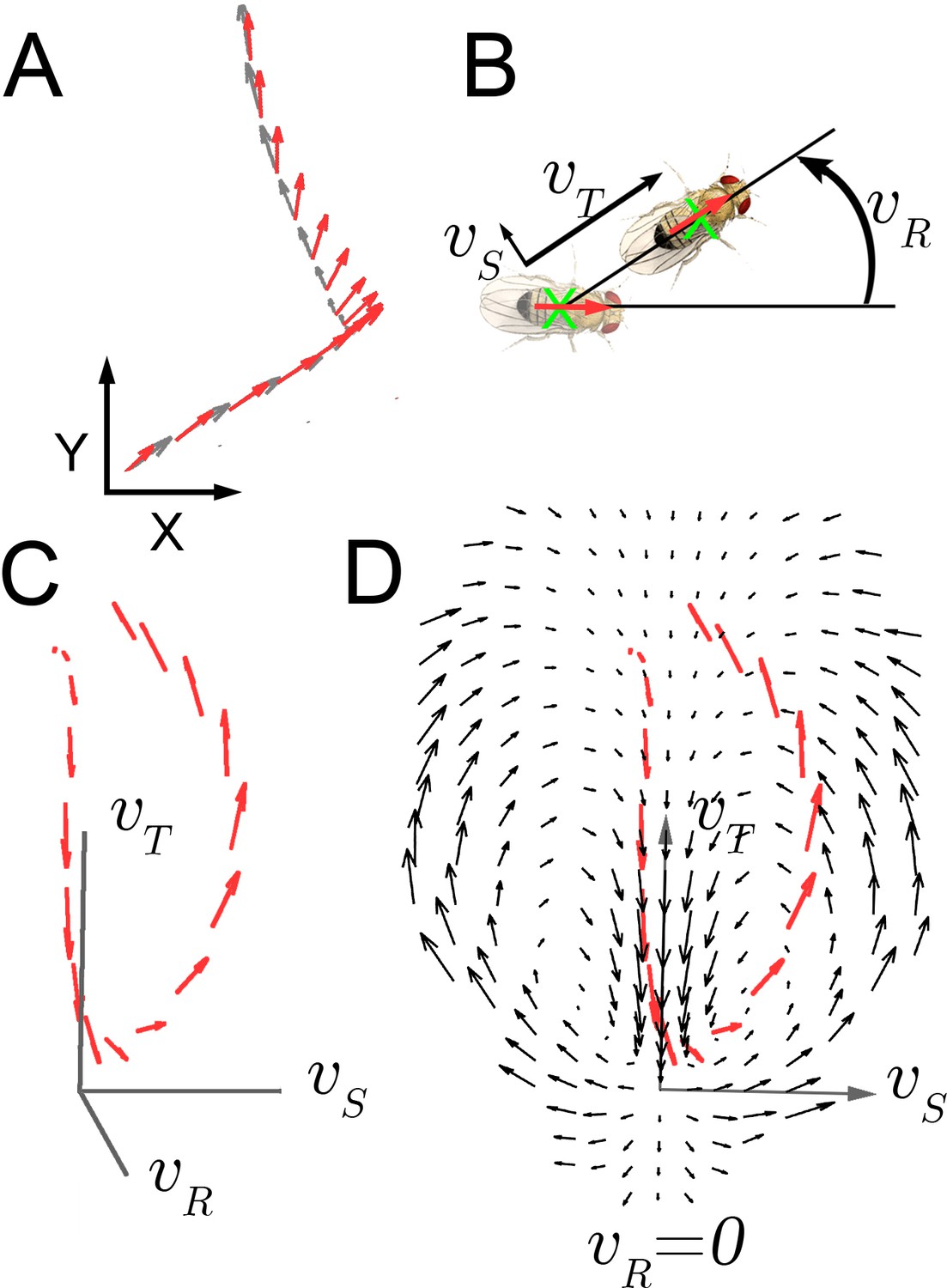
Velocity-acceleration phase space captures aggregate constraints on behavior.

(A) An example trajectory fragment of an individual fly walking on a surface. The animal’s orientation (red arrows) and displacement (gray arrows) are tracked at 30 frames per second. (B) A schematic illustration of the three velocity components $\vec{v} = (v_{T}, v_{R}, v_{S})$ around the major body axis of a fly. These three components completely describe whole-animal movement in two dimensions. (C) Example trajectory in velocity phase space parameterized by $\vec{v} = (v_{T}, v_{R}, v_{S})$ . Red arrows denote the magnitude of the acceleration vector at each velocity. (D) A single plane in the 3-dimensional phase space, $E [\dot{\vec{v}} ∣ \vec{v}], \vec{v} = (v_{T}, v_{R} = 0, v_{S})$ (black arrows), with an example trajectory (red arrows), projected into this plane (x-axis: $v_{S}$ ; y-axis: $v_{T}$ ).

https://doi.org/10.7554/eLife.26410.002

Figure 2

Download asset Open asset

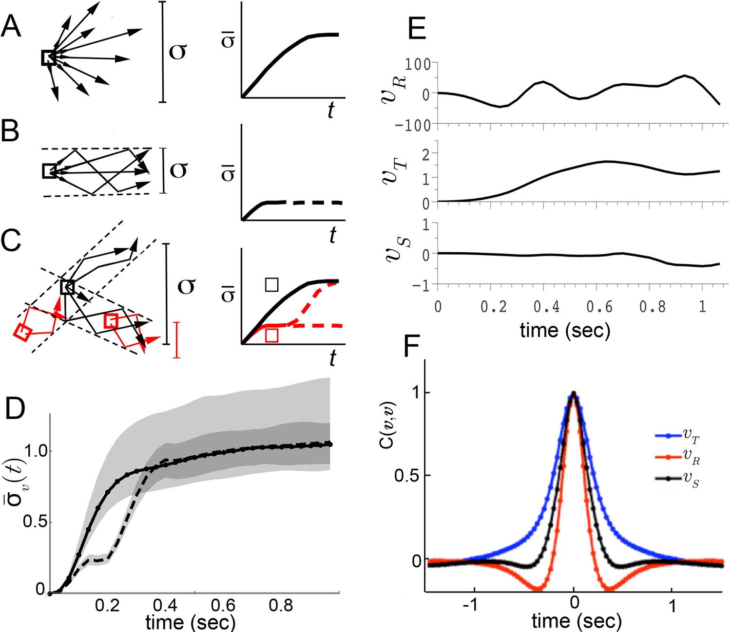
Trajectory divergence in velocity phase space and definition of a behavior episode around $v_{R}$ extrema.

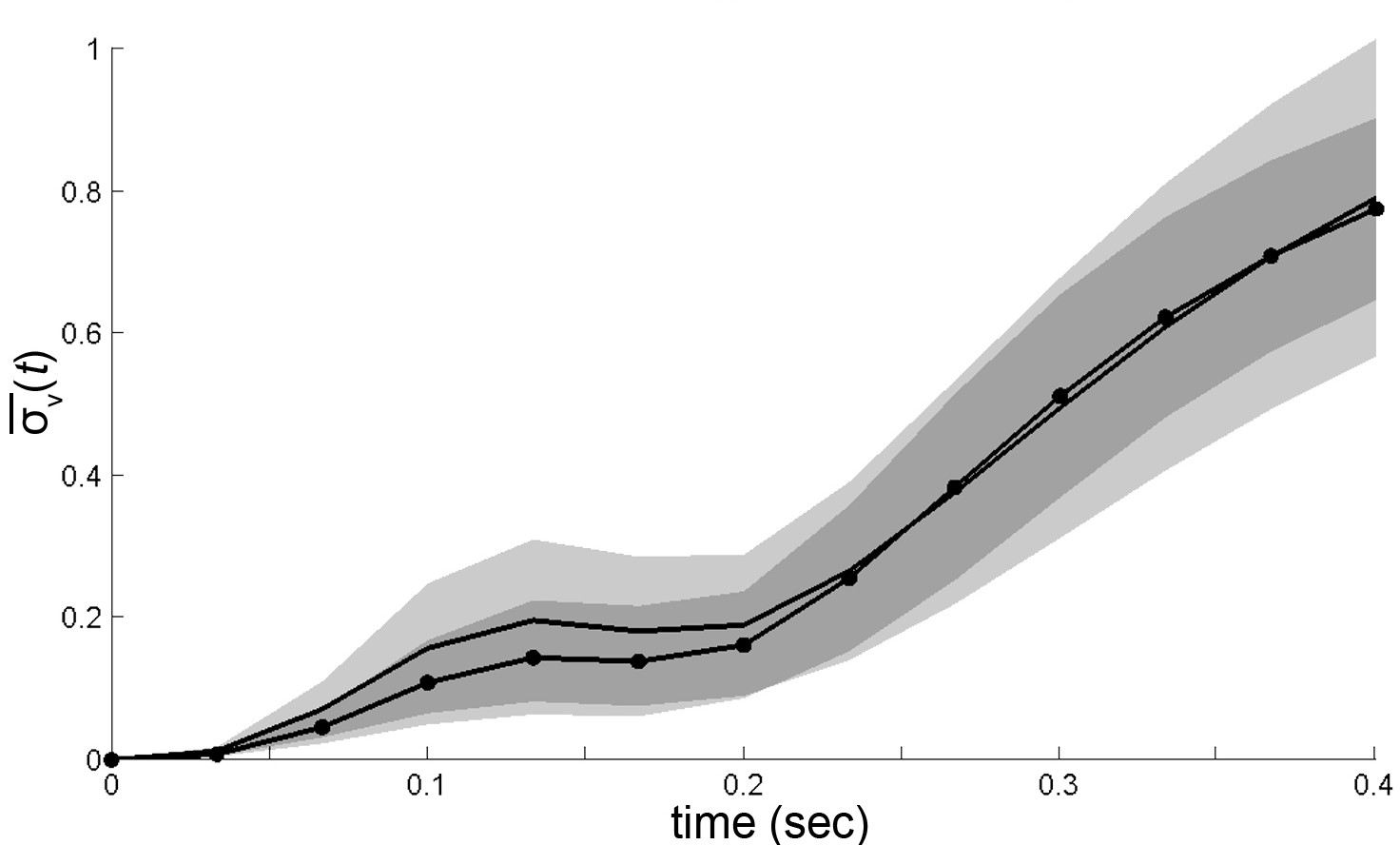
(A) Starting from a small neighborhood of similar velocities (box), diverging trajectories spread throughout velocity phase space, increasing in a measure of their spread. (B) Starting from the same neighborhood, divergence of trajectories corresponding to modal patterns is bounded for the duration of each pattern. (C) Bounded or unbounded divergence can be seen when modal patterns overlap in velocity phase space, depending on when trajectories are sampled in the course of these patterns. (D) The normalized standard deviation of trajectories at time $t$ after passage through a small neighborhood, averaged over a random sample of $N_{B} = 200$ neighborhoods, $\bar{σ} (t) = \frac{1}{σ [v_{T}] σ [v_{R}] σ [v_{S}]} ⟨ σ_{t} [v_{T}] σ_{t} [v_{R}] σ_{t} [v_{S}] ⟩_{N_{B}}$ (Equation 1, Materials and methods). Shaded areas represent 95% confidence intervals of the estimate of $\bar{} (t)$ . Neighborhoods were sampled from anywhere in velocity space, and for each neighborhood all trajectories were included (dot-solid line), or only those with a turn peak 100 ms after passing the neighborhood (dashed line). (E) An example trajectory fragment depicting $v_{R} (τ)$ [° s⁻¹], $v_{T} (τ)$ and $v_{S} (τ)$ [cm s⁻¹]. (F) The autocorrelation functions of $v_{R} (τ), v_{T} (τ)$ and $v_{S} (τ)$ .

https://doi.org/10.7554/eLife.26410.003

Figure 3

Download asset Open asset

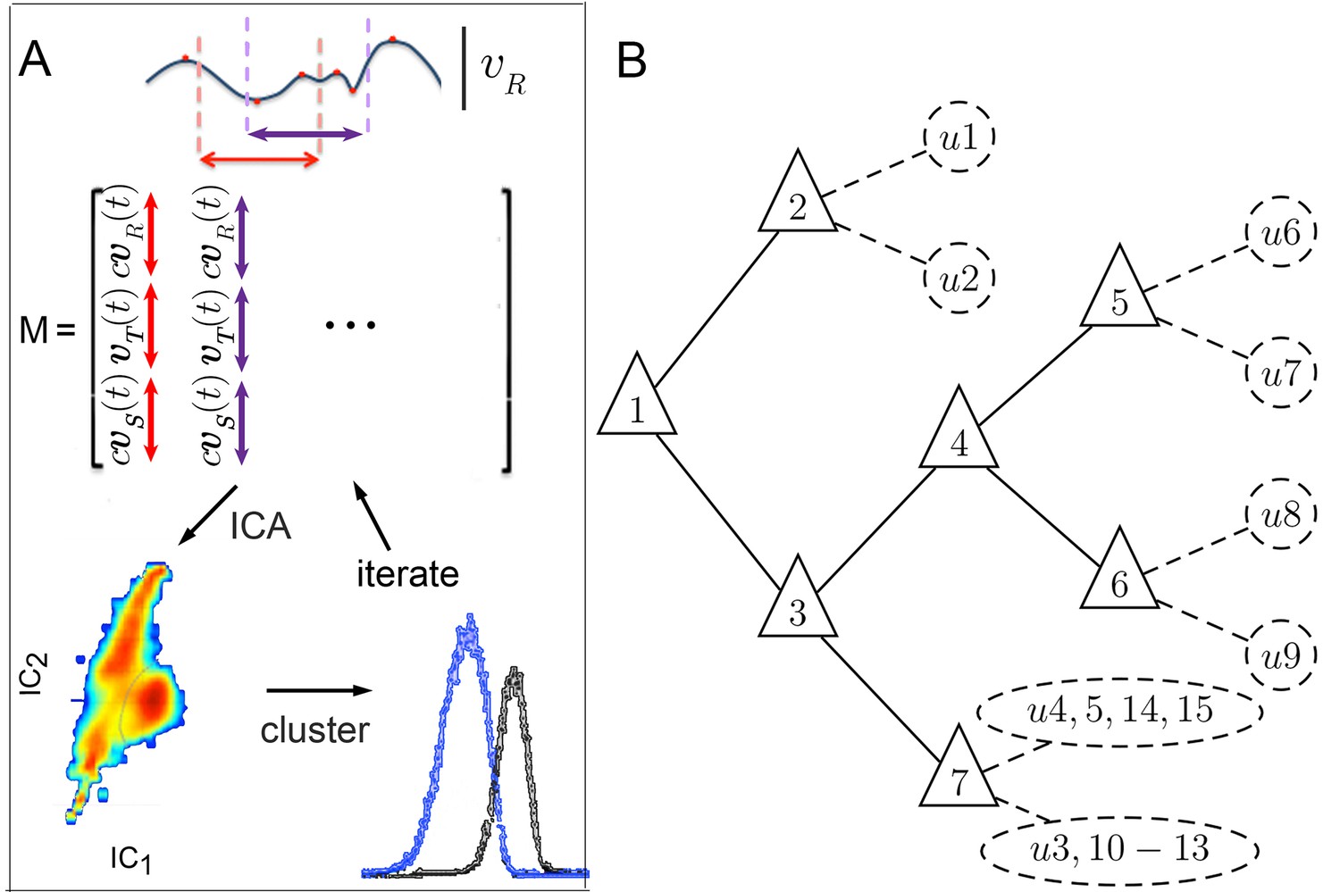
Iterative ICA segmentation reveals dynamic submodes.

(A) Iterative ICA procedure. Local $v_{R}$ peaks are identified in a single trajectory (red dots). Fragments of trajectories are then selected around $v_{R}$ (dashed lines), and all velocity components are aligned in time on $v_{R}$ extrema in matrix $M$ . In $M$ , turn direction is normalized while preserving the relative direction of side slip by multiplying $v_{R}$ and $v_{S}$ by $c$ , the sign of $v_{R}$ extremum at aligned time 0. $M$ dimensionality is then reduced and independent components are identified. In these independent components, velocity trajectories are represented by a coefficient in each component. If a multimodal coefficient distribution is found, coefficient clusters corresponding to distinct trajectory fragment subsets are separated, and the entire procedure is repeated iteratively on each fragment subset to identify distinct submodes. (B) Segmentation tree showing decision points (triangles), and submodes (dashed circles). 15 submodes were identified, but the decision tree is drawn up to branching levels supported by Markov modeling (Figure 5, Figure 5—figure supplement 1). Submodes are described in Figure 4 and Figure 4—figure supplement 1.

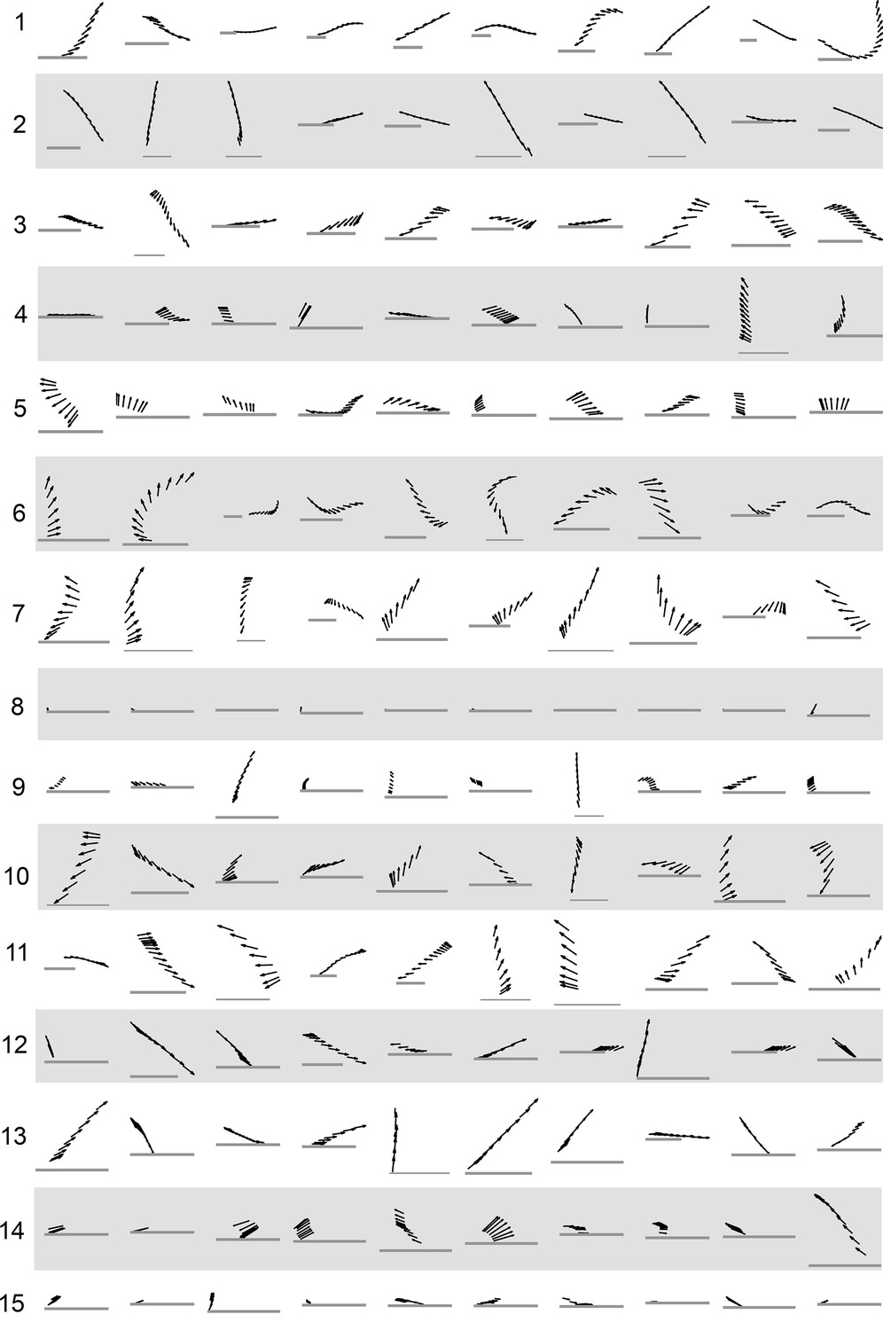
https://doi.org/10.7554/eLife.26410.004

Figure 4 with 1 supplement

Download asset Open asset

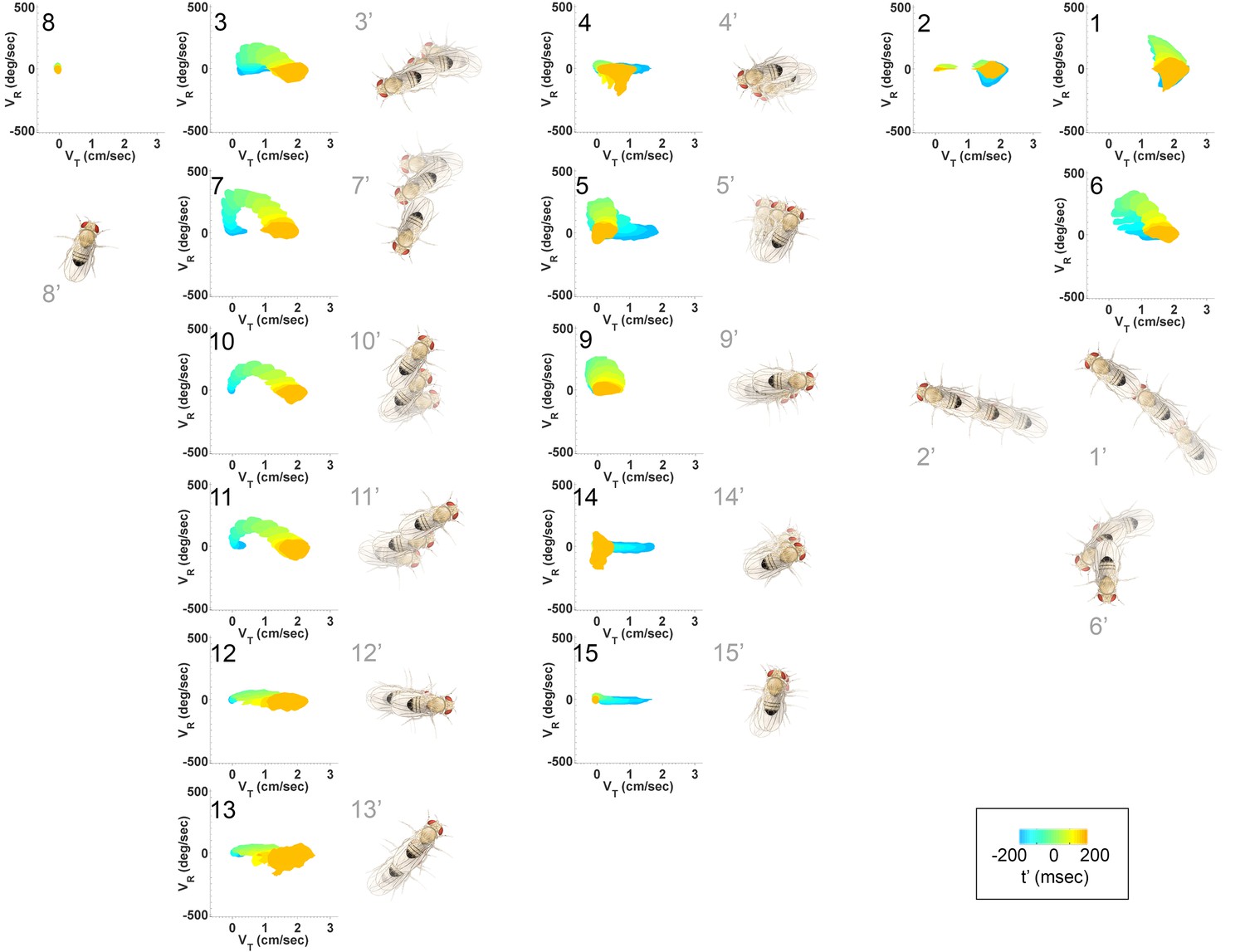
Submode velocity profiles for each submode.

(1-15) Velocity distributions over time for each identified submode. The central 68% of the distribution is shown at each time point for up to 200 ms around peak $v_{R}$ . The time within each submode relative turn peak is color-coded. Submodes are shown in columns, by membership in modes $I - V$ (Figure 5). (1’−15’) Example trajectory fragment of each submode type is illustrated. Three time points are shown per trajectory, each spaced 100 ms apart. A diagrammed fly illustrates the centroid location and orientation of an animal at each time point. Note that only one time point illustrates submode 8 because this submode consists of stops.

https://doi.org/10.7554/eLife.26410.007

Figure 4—figure supplement 1

Download asset Open asset

Example trajectory fragments from each submode class.

Black arrows represent a fly’s body orientation, shown at 33 time steps. Gray horizontal scale bars = 3 mm, a representative length of an adult *D. melanogaster* female. Ten samples from each submode were drawn randomly. The time interval shown is between the two acceleration peaks flanking each submode, taken as a period between behavior adjustments as described in Main Text.

https://doi.org/10.7554/eLife.26410.008

Figure 5 with 2 supplements

Download asset Open asset

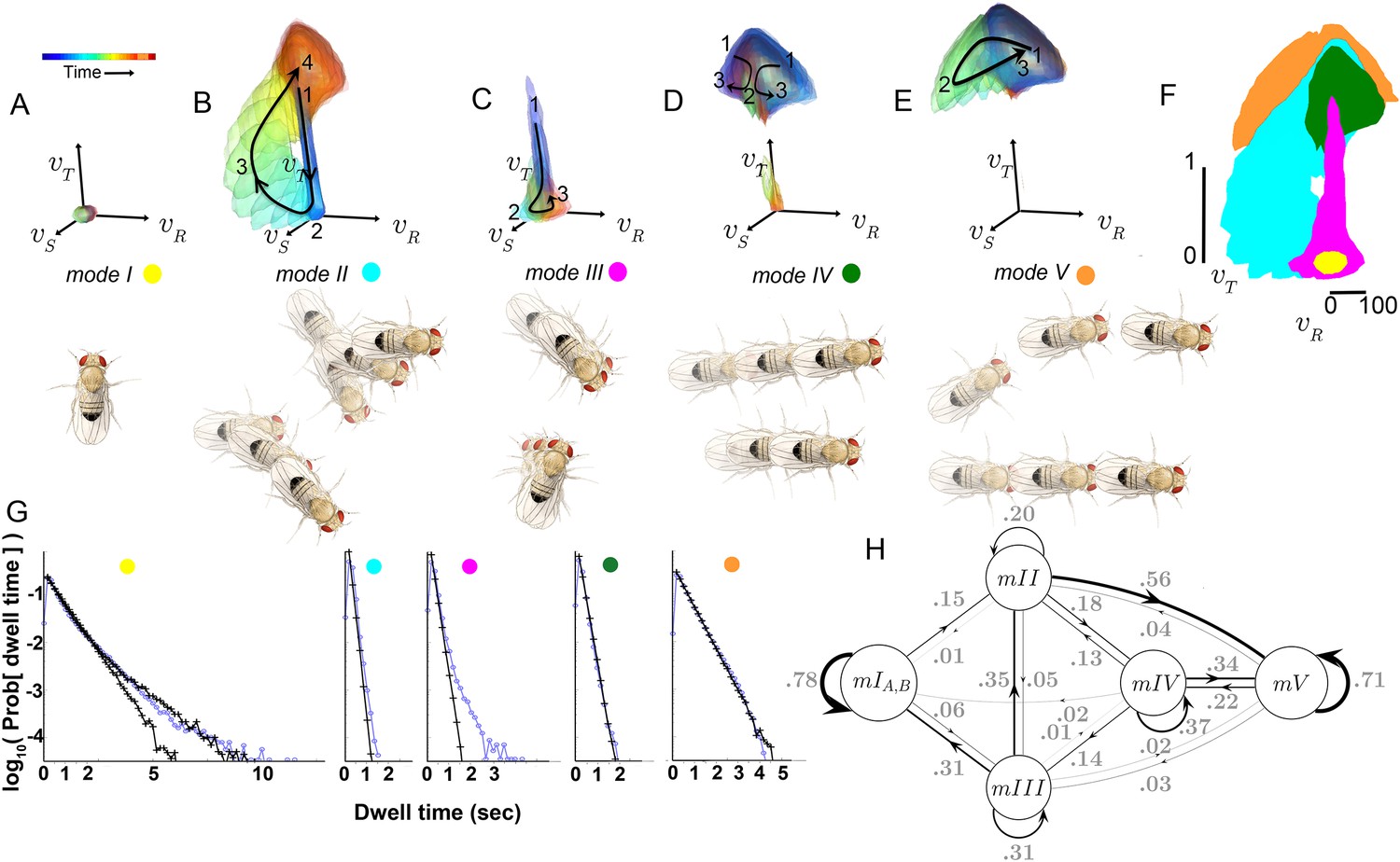
Identified movement patterns as distributions in velocity phase space.

(**A–E**) Top: Modes are described as velocity distributions over time, termed ‘velocity profiles.’The central 68% of the velocity distribution at each time point around peak $v_{R}$ is shown. The time relative to a turn peak within each mode is color-coded; green represents time of peak $v_{R}$ . Bottom: Example trajectory fragments from each mode are illustrated. Except for $M o d e I$ , two trajectories are shown per mode, three time points per trajectory, each spaced 100 ms apart. A diagrammed fly illustrates the centroid location and orientation of an animal at each time point. Note that only one time point illustrates $M o d e I$ because this mode consists of stops. (F) Projection of all mode velocity profiles into a $v_{T} - v_{R}$ plane. Note that modes overlap in this joint velocity projection, and modes spanning smaller velocity regions are plotted on top of broader modes. (G) Residence time distributions, by mode, from real (light blue) and model-generated (black) trajectories. Two model-generated distributions are plotted for $m o d e I$ (left panel): a Markov model without hidden states captures short residence times in the real distribution, while a Markov model that included an additional, non-communicating hidden state captures both short and long residence times. (H) The chosen 5-state Markov model, $M M 5$ . Edges are labeled with transition probabilities between modes. This model does not represent hidden substates of $m o d e I$ .

https://doi.org/10.7554/eLife.26410.009

Figure 5—figure supplement 1

Download asset Open asset

Grouping submodes by kinetic criteria to define a behavioral model.

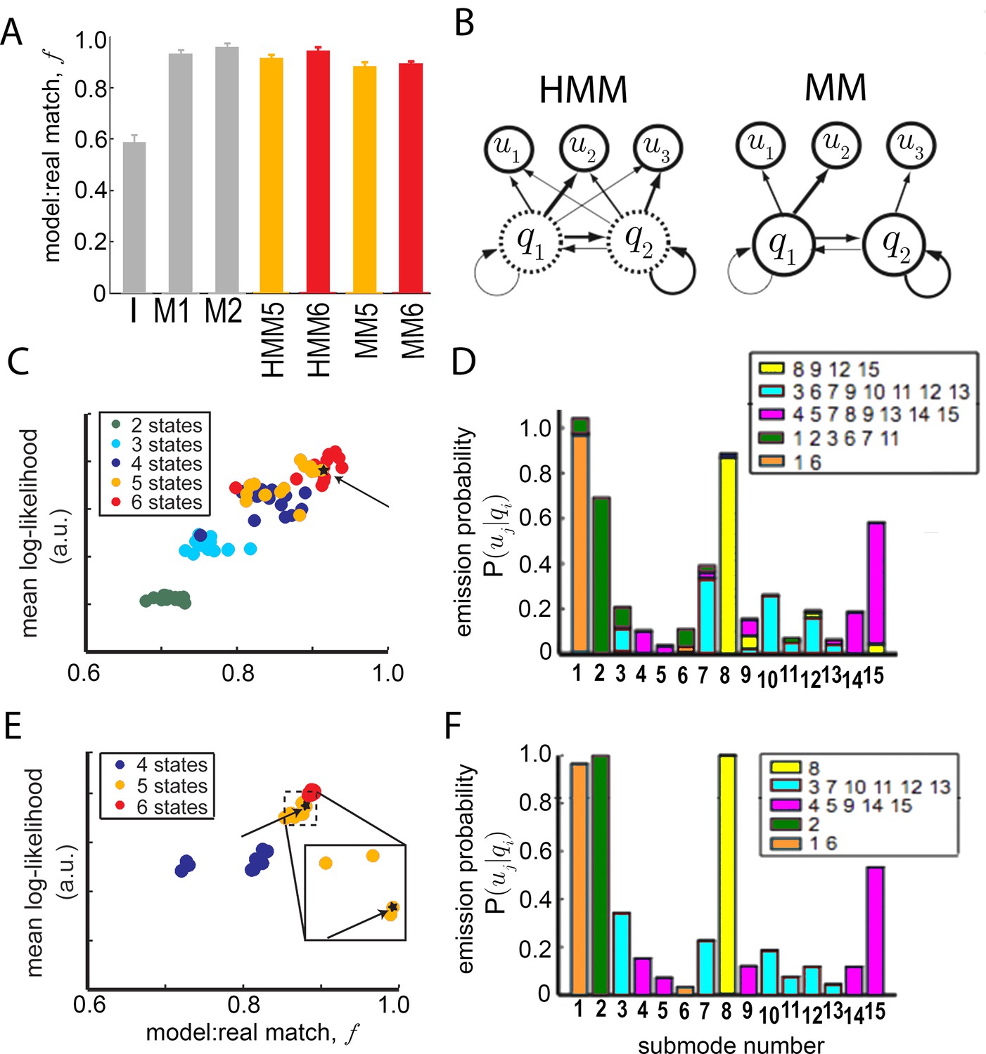
(A) Statistical relationship of submodes assessed using sampling from generative models. Short trajectory fragments generated using statistics from all 15 submodes individually (gray bars) or submode groups (orange, red bars) were compared to real trajectory fragments ( $m e a n \pm s . d .$ duration = $1.3 \pm 0.3$ sec). To generate synthetic sequences, submode transition statistics were either estimated directly from submode sequences in real trajectories (models I,M1,M2), and then used to generate synthetic submode sequences, or transition statistics from state model fits to data were first used to generate state sequences, and then emission statistics fit by each model were used to sample submodes associated with each state, producing submode sequences (HMM,MM). In all cases, submode sequences were compared between real and model-generated sets of sequences. The matched fraction $(f)$ of real sequences, quantifying set overlap, is the average number of exact matches between synthetic and real fragment sets, normalized by the average number of matches between two randomly sampled real sets (Materials and methods sections IV and V, Equation 10). First- and second-order Markov models (M1,M2) perform significantly better than a model that presumes independence between submodes (I) $(f_{I} = 0.58 \pm 0.016; f_{M 1} = 0.93 \pm 0.009; f_{M 2} = 0.96 \pm 0.008)$ . Five and six state Hidden Markov Models (HMM5,6), as well as 5 and 6 state Markov Models (MM5,6) without hidden states perform well on this generative test $(f_{H M M 5} = 0.91 \pm 0.007; f_{H M M 6} = 0.94 \pm 0.009; f_{M M 5} = 0.88 \pm 0.010; f_{M M 6} = 0.89 \pm 0.006)$ . (B) Illustration of the relevant difference between HMM and MM: in a MM (right) observable submodes $(u_{1}, u_{2}, u_{3})$ unambiguously reflect an underlying state $q_{i}$ (termed a $M o d e, m_{i}$ ). In an HMM (left) a given observed submode $u_{j}$ may arise from more than one underlying state $q_{i}$ . (C) HMM mean log-likelihood values, plotted against performance on a generative test (fragment set matched fraction, $f$ ). Each HMM is represented by a dot and colored by the number of hidden states. (D) Emission probabilities, $\Pr [s u b m o d e u_{j} ∣ s t a t e q_{i}]$ for a selected 5-state HMM (HMM5, starred in C). Bar colors represent emitting state $q_{i}$ . Legends list the submodes associated with each state. These are submodes $u$ for which $\Pr [u_{j} ∣ q_{i}]$ is significantly higher than 0. (E) MM performance on likelihood and generative tests as in (C). (F) Emission probabilities, $\Pr [s u b m o d e u_{j} ∣ s t a t e q_{i} = M o d e m_{i}]$ , for the selected MM (MM5, starred in E, and E inset). Modes are colored as in Figure 5.

https://doi.org/10.7554/eLife.26410.010

Figure 5—figure supplement 2

Download asset Open asset

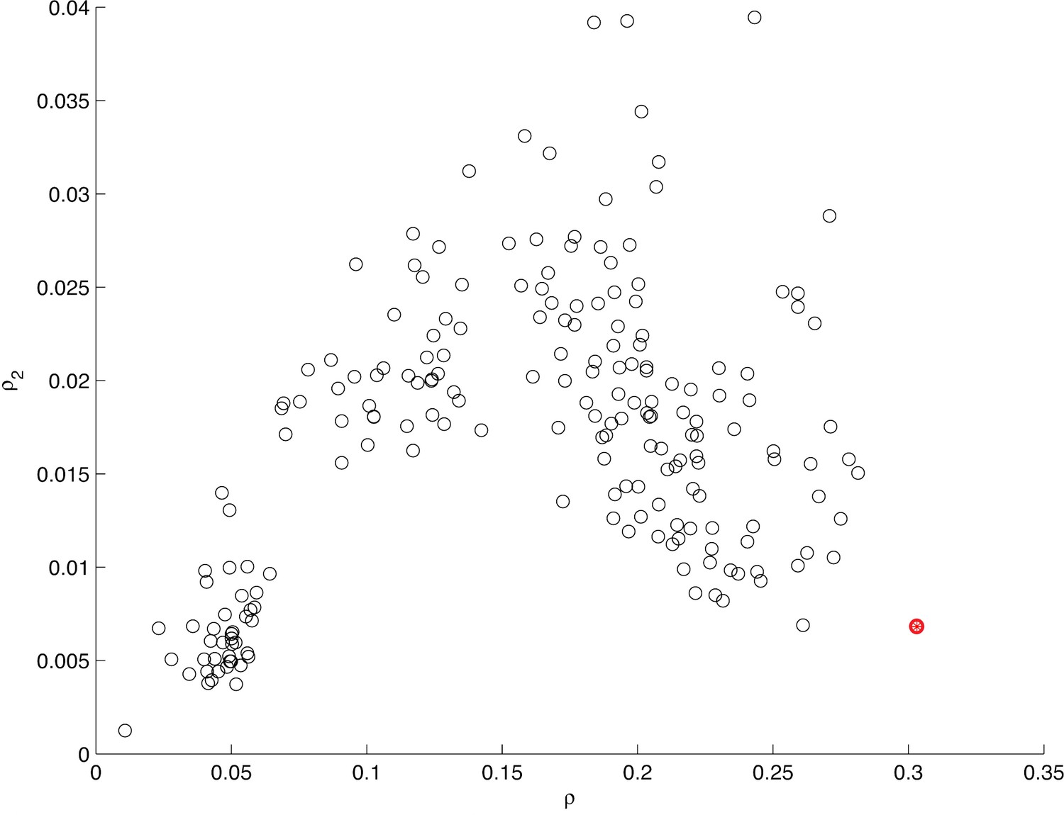
Information between modes in sequences.

The fraction of uncertainty about mode identity in sequences, explained by the previous mode $(ρ)$ and the mode before that $(ρ_{2})$ , plotted for different arbitrary models that group submodes into five groups in different ways. Each circle represents a unique grouping. The result of the actual grouping identified in Figure 5—figure supplement 1, in MM5, is shown in red. For mode sequences of any length $k > 2, {(m_{i})}_{i = 1}^{k}, m \in {I \dots V}, ρ = I (m_{i}; m_{i - 1}) / H (m)$ and $ρ_{2} = I (m_{i}; m_{i - 2} ∣ m_{i - 1}) / H (m_{i} ∣ m_{i - 1})$ , where $I$ is mutual information and $H$ is Shannon entropy (Cover and Thomas, 1991).

https://doi.org/10.7554/eLife.26410.011

Figure 6 with 1 supplement

Download asset Open asset

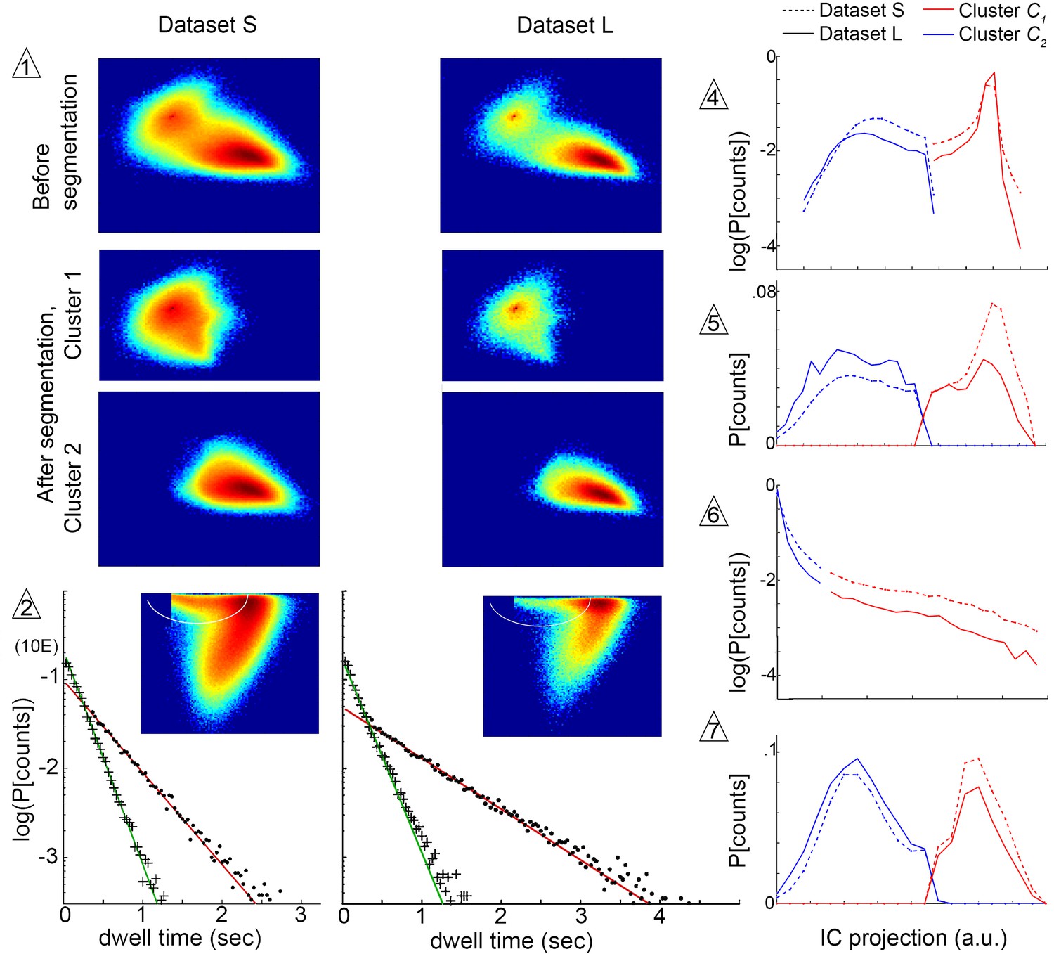
Submode segmentation in two datasets, S and L.

Histograms of trajectory coefficients $s^{(j)}$ in independent component space (Box 1 and Materials and methods) are shown at decision points of the iterative segmentation procedure. Heat maps show counts in two dimensions of the independent component space, and line plots show counts in one dimension. Decision points (numbered triangles) correspond to decision points labeled on the segmentation tree in Figure 3B. Subsets of coefficients separated at each decision point are shown in the same dimensions, as noted. Plot dimensions do not necessarily correspond to independent components, as sometimes data was rotated in IC space to visualize multimodal coefficient distributions. Trajectories from two different experimental conditions, corresponding to datasets S and L, were projected in the same independent components, and their coefficients are shown on the same or adjacent plots, as noted below. The initial decision point (1) and all terminal decision points (2,4–7) are shown. The coefficient distribution at decision point three is not shown because it could not be represented in two dimensions. Decision pt. (1). $^{(j)}$ histograms in two dimensions, showing the multimodal distribution of coefficients from the entire dataset (Top plots), and coefficient clusters 1 and 2 after they were separated at this decision point (Bottom plots). Decision pt. (2) Data projection in two dimensions before segmentation, showing the segmentation cut (white oval), and the dwell time distributions for each resulting submode, along with single exponential fits. Note that dwell time distributions are consistent with one dominant component for each segmented submode, despite differences in the joint velocity distributions and dwell times between datasets S and L. Decision pts. (4-7) $s^{(j)}$ histograms in one dimension, as used for segmentation. Note that the distribution at decision point six is plotted on a log scale, where segmentation separates the long tail. Decision pt. seven is upstream of further segmentations that were not validated by Markov models. As these submodes are very low frequency, they may represent distinct submodes that can be validated using larger datasets. The 5-state MM5 groups submodes as follows: $M o d e I : u_{8}; M o d e I I : u_{7}, u_{3}, u_{10 - 13}; M o d e I I I : u_{9}, u_{4}, u_{5}, u_{14 - 15};$ $M o d e I V : u_{2}; M o d e V : u_{1}, u_{6}$ .

https://doi.org/10.7554/eLife.26410.013

Figure 6—figure supplement 1

Download asset Open asset

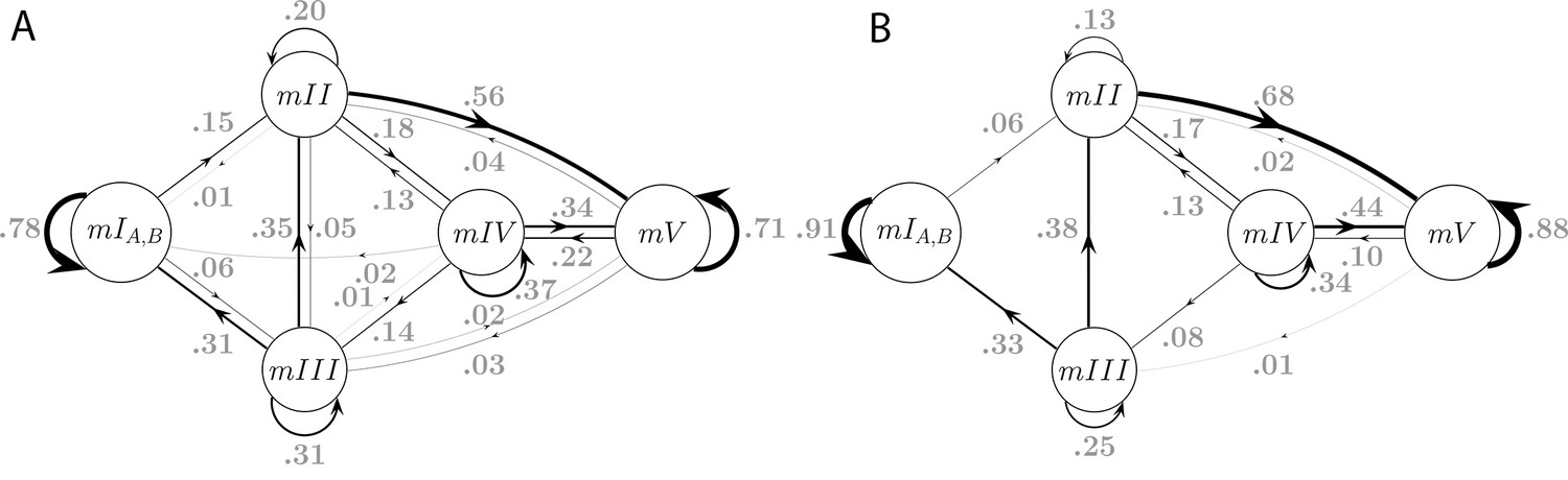
Model connectivity and transition frequencies in two datasets.

Transition probabilities of the 5-state Markov Model MM5 are shown for dataset S (A, same as Figure 5H), and dataset L (B).

https://doi.org/10.7554/eLife.26410.014

Figure 7 with 2 supplements

Download asset Open asset

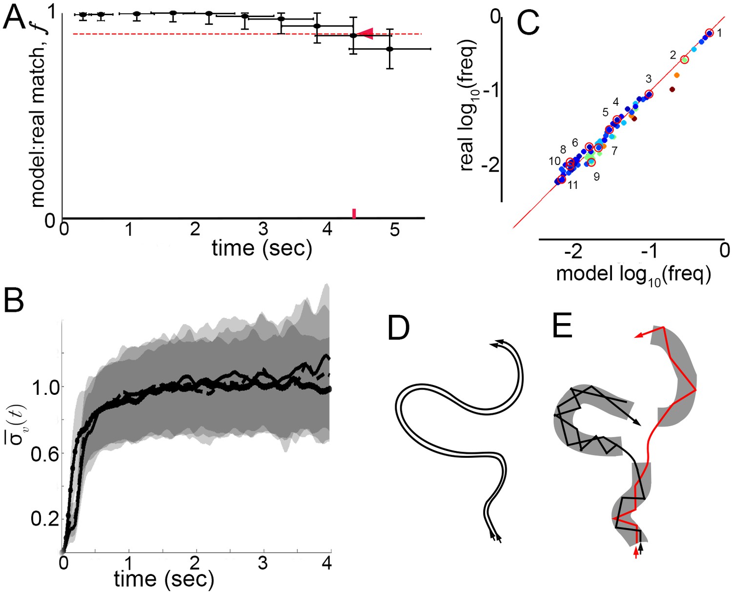
Model prediction and trajectory divergence over time.

(A) Matched fraction $(f)$ of mode sequences from real trajectories as a function of sequence length. Synthetic mode sequences were generated using the transition component of the model MM5. Red dashed line marks $f = 90 %$ , red tick and arrow mark the sequence length when $f$ first crosses below 90%. (B) Trajectory divergence in velocity space from randomly sampled small neighborhoods, without and with information about current mode identity. Two divergence curves from Figure 2D are replotted over a longer time scale: starting from neighborhoods anywhere in velocity space, and including all trajectories (dot-solid line), or including only trajectories that attained a turn peak 100 ms later(dashed line), or only those with a turn peak 100 ms later corresponding to a given mode (solid line). Dashed and solid lines overlap for their durations. Note the short $\bar{}$ plateau, and rise after approximately 200 ms. (C) Predicted versus actual log-frequency of all mode sequences above measurement noise, up to trajectories that include 17 consecutive modes, covering 4.3 s. Markers are colored by sequence length, from shortest (2-mer, dark blue) to longest (17-mer, dark red). $R = 1.00, n = 60, p ≪ 0.001$ ; Sampling error cutoff is at $f r e q < \frac{1}{2} (2.58 N^{- \frac{1}{2}})$ , $N$ = number of sequences in each condition. Ten of these sequences (#2–11) were randomly selected for display in Figure 7—figure supplement 1, plus the most common sequence (#1). (D) Illustration of velocity trajectories specified by a stable dynamical system. Two trajectories starting from similar velocities (arrowheads, bottom), follow similar paths over time that show little divergence some time later (arrowheads, top). (E) Illustration of mode structure and transitions in velocity space. Trajectories from a small region of velocity phase space (black and red arrows) display bounded divergence for the duration of a mode (gray area) but display approximately no memory of past behavior at transitions (gaps between gray regions) beyond their current mode. Note divergence in the course of mode traversal may lead to path scrambling inside modes (jagged lines).

https://doi.org/10.7554/eLife.26410.017

Figure 7—figure supplement 1

Download asset Open asset

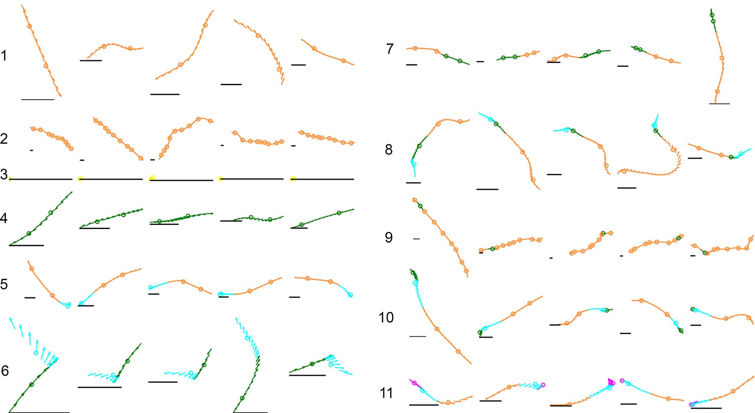
Examples of common mode sequences.

Arrows represent a fly’s body orientation, shown at 33 time steps. Examples are colored by membership in a mode class of Markov model MM5, with each mode center marked by a circle on the trajectory. Gray horizontal scale bars = 3 mm, a representative length of an adult *D. melanogaster* female. Numbers reference locations in Figure 5C, ascending from the most common to the rarest sequence shown.

https://doi.org/10.7554/eLife.26410.018

Figure 7—figure supplement 2

Download asset Open asset

Trajectory divergence in velocity space, measured from the center or periphery of each mode’s velocity distribution.

Trajectory divergence from small neighborhoods in velocity space (occupying 0.004% of space) was measured separately by mode, and by each neighborhood’s quartile in that mode’s velocity distribution $Pr [v_{T}, v_{R}, v_{S} ∣ t^{'}]$ , at $t^{'} = - 100$ ms. Divergence from individual neighborhoods was then averaged in the center $(P_{25.5 - 74.5})$ and in the periphery $(P_{1 - 25.5} and P_{74.5 - 99})$ for all modes (*center*, dot-solid line; *periphery*, solid line). Shaded areas represent 95% confidence intervals for estimates of $\bar{} (t)$ .

https://doi.org/10.7554/eLife.26410.019

Tables

Table 1

Transition rates ${[T r]}_{i j}$ , dataset S (uniform illumination, test tubes). Rows: ‘From’ mode; Columns: ‘To’ mode. Transitions below sampling error are gray.

https://doi.org/10.7554/eLife.26410.012

	I	II	III	IV	V
I	0.7764	0.1572	0.0608	0.0037	0.0020
II	0.0058	0.2010	0.0521	0.5598	0.1812
III	0.3129	0.3464	0.3082	0.0227	0.0098
IV	0.0029	0.0353	0.0349	0.7111	0.2159
V	0.0248	0.1298	0.1364	0.3422	0.3668

Table 2

Comparison of transition velocity profiles between datasets S and L. Overlap between mode velocity profiles is shown by transition type, comparing modes in datasets S and L. 1 = perfect overlap; 0 = no overlap. Rows: ‘From’ mode; Columns: ‘To’ mode. Gray values fail significance criteria as reported in Table 3.

https://doi.org/10.7554/eLife.26410.015

	I	II	III	IV	V
I	1.00	0.97	0.96	0.83	0.83
II	0.76	0.94	0.89	0.93	0.96
III	0.99	0.95	0.95	0.87	0.82
IV	0.89	0.94	0.95	0.94	0.97
V	0.99	0.96	0.97	0.97	0.99

Table 3

Probability that dataset L and S transitions are drawn from the same velocity profiles, by bootstrap for each transition type. $p < 0.002$ is significant at $P r o b < 0.05$ level, using Bonferroni correction for 25 independent comparisons.

https://doi.org/10.7554/eLife.26410.016

	I	II	III	IV	V
I	0.0001	0.0001	0.0001	0.2354	0.4162
II	0.1739	0.0001	0.0001	0.0002	0.0001
III	0.0001	0.0002	0.0002	0.0003	0.0901
IV	0.0138	0.0001	0.0001	0.0001	0.0001
V	0.0284	0.0001	0.0001	0.0001	0.0001

Table 4

Materials and methods – Supplementary table 1. Comparison of dataset parameters, measurements, and findings.

https://doi.org/10.7554/eLife.26410.020

Work	Fly strain	Gender	Age (days,p. e.)	Recording Duration(min)	Fly speed (median,cm/sec) ^[c]	Measure-ment	Segmented behaviors, Total	Segmented behaviors, Locomotor
Berman et al. ^[a]	Oregon-R	♂, ♀	1-14	60	0.3 (♂)	2-D image (posture)	117	17
Berman et al. ^[b]	.	♂	.	.	.	.	.	.
Katsov et al.	Oregon-R	♀	2-3	10	2.0	body velocity	15	15^[d]

[ . ] same value as row above.
[a] (Berman et al., 2014)
[b] (Berman et al., 2016)
[c] Berman et al. (2014) show median velocity ~0.3 mm/sec (Fig S1); the units appear to be a typographical error.
[d] Count includes submode 8/mode I, a mixture of locomotor and non-locomotor states (stops).