SynEM, automated synapse detection for connectomics
- Max Planck Institute for Brain Research, Germany
- Biomimetic Robotics and Machine Learning, Germany
Figures
Figure 1
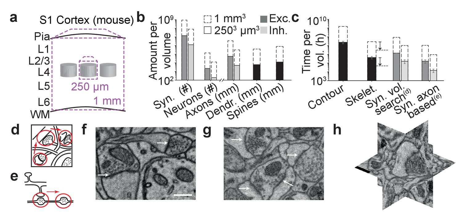
The challenge of synapse detection in connectomics.
(a) Sketch of mouse primary somatosensory cortex (S1) with circuit modules (‘barrels’) in cortical layer 4 and minimum required dataset extent for a ‘barrel’ dataset (250 µm edgelength) and a dataset extending over the whole cortical depth from pia to white matter (WM) (1 mm edge length). (b) Number of synapses and neurons, total axonal, dendritic and spine path length for the example datasets in (a) (White and Peters, 1993; Braitenberg and Schüz, 1998; Merchán-Pérez et al., 2014). (c) Reconstruction time estimates for neurites and synapses; For synapse search strategies see sketches in d,e. Dashed arrows: latest skeletonization tools (webKnossos, Boergens et al., 2017) allow for a further speed up of neurite skeletonization by about 5-to-10-fold, leaving synapse detection as the main annotation bottleneck. (d) Volume search for synapses by visually investigating 3d image stacks and keeping track of already inspected locations takes about 0.1 h/µm3. (e) Axon-based synapse detection by following axonal processes and detecting synapses at boutons consumes about 1 min per bouton. (f) Examples of synapses imaged at an in-plane voxel size of 6 nm and (g) 12 nm in conventionally en-bloc stained and fixated tissue (Briggman et al., 2011; Hua et al., 2015) imaged using SBEM (Denk and Horstmann, 2004). Arrows: synapse locations. Note that synapse detection in high-resolution data is much facilitated in the plane of imaging. Large-volume image acquisition is operated at lower resolution, requiring better synapse detection algorithms. (h) Synapse shown in 3D EM raw data, resliced in the 3 orthogonal planes. Scale bars in f and h, 500 nm. Scale bar in f applies to g.
-
Figure 1—source data 1
Source data for plots in panels 1b, 1c.
- https://doi.org/10.7554/eLife.26414.004
Figure 2
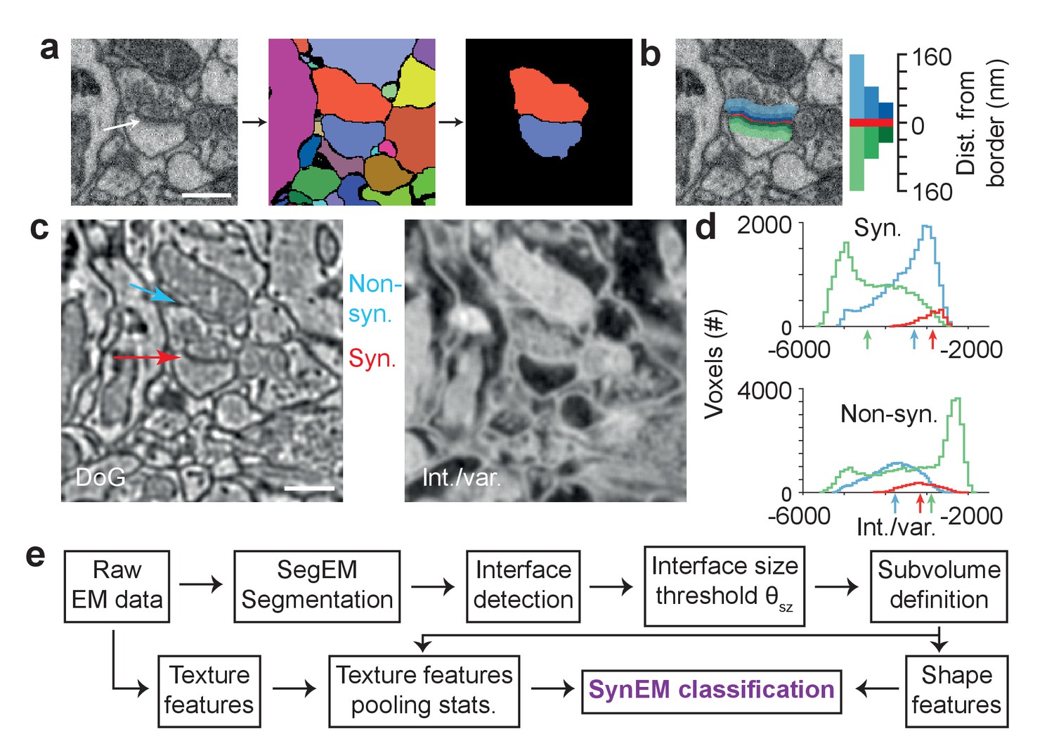
Synapse detection by classification of neurite interfaces.
(a) Definition of interfaces used for synapse classification in SynEM. Raw EM data (left) is first volume segmented (using SegEM, Berning et al., 2015). Neighboring volume segments are identified (right). (b) Definition of perisynaptic subvolumes used for synapse classification in SynEM consisting of a border (red) and subvolumes adjacent to the neurite interface extending to distances of 40, 80 and 160 nm. (c) Example outputs of two texture filters: the difference of Gaussians (DoG) and the intensity/variance filter (int./var.). Note the clear signature of postsynaptic spine heads (right). (d) Distributions of int/var. texture filter output for image voxels at a synaptic (top) and non-synaptic interface (bottom). Medians over subvolumes are indicated (arrows, color scale as in b). (e) SynEM flow chart. Scale bars, 500 nm. Scale bar in a applies to a,b.
-
Figure 2—source data 1
Source data for plot in panel 2d.
- https://doi.org/10.7554/eLife.26414.006
Figure 3 with 4 supplements

SynEM training and evaluation.
(a) Histogram of SynEM scores calculated on the validation set. Fully automated synapse detection is obtained by thresholding the SynEM score at threshold θ. (b) SynEM scores for the two possible directions of interfaces. Note that SynEM scores are disjunct in a threshold regime used for best single synapse performance (θs) and best neuron-to-neuron recall and precision (θnn), see Figure 5, indicating a clear bias towards one of the two possible synaptic directions. (c) Strategy for label generation. Based on annotator labels (Ann. Label), three types of label sets were generated: Initial label set ignored interface orientation (Undir.); Augmented label set included mirror-reflected interfaces (Augment.); Directed label set used augmented data but considered only one synaptic direction as synaptic (Directed, see also Figure 3—figure supplement 1). (d) Development of the SynEM classifier. Classification performance for different features, aggregation statistics, classifier parameters and label sets. Init: initial classifier used (see Table 1). The initial classifier was extended by using additional features (Add feat, see Table 1, first row), 40 and 80 nm subvolumes for feature aggregation (Add subvol, see Figure 2b) and aggregate statistics (Add stats, see Table 1). Direct: Classifier trained on directed label set (see Figure 3c). Logit: Classifier trained on full feature space using LogitBoost. Augment and Logit: Logit classifier trained on augmented label set (see Figure 3c). Direct and Logit: Logit classifier trained on directed label set (see Figure 3c). (e) Test set performance on 3D SBEM data of SynEM (purple) evaluated for spine and shaft synapses (all synapses, solid line) and for spine synapses (exc. synapses, dashed line), only. Threshold values for optimal single synapse detection performance (black circle) and an optimal connectome reconstruction performance (black square, see Figure 5). (see also Figure 3—figure supplement 2) (f) Relation between 3D EM imaging resolution, imaging speed and 3D EM experiment duration (top), exemplified for a dataset sized 1 mm3. Note that the feasibility of experiments strongly depends on the chosen voxel size. Bottom: published synapse detection performance (reported as F1 score) in dependence of the respective imaging resolution (see also Supplementary file 1). dark blue, Mishchenko et al. (2010); cyan, Kreshuk et al. (2011); light gray, Becker et al. (2012); dark gray, Kreshuk et al. (2014); red, Roncal et al. (2015); green, Dorkenwald et al. (2017); Black brackets indicate direct comparison of SynEM to top-performing methods: SynEM vs Roncal et al. (2015) on ATUM-SEM dataset (Kasthuri et al., 2015); SynEM vs Dorkenwald et al. (2017) and Becker et al. (2012) on our test set. See Figure 3—figure supplement 3 for comparison of Precision-Recall curves. Note that SynEM outperforms the previously top-performing methods. Note also that most methods provide synapse detection, but require the detection of synaptic partners and synapse direction in a separate classification step. Gray solid line: drop of partner detection performance compared to synapse detection in Dorkenwald et al. (2017); dashed gray lines, analogous possible range of performance drop as reported for bird dataset in Dorkenwald et al. (2017). SynEM combines synapse detection and partner detection into one classification step.
-
Figure 3—source data 1
Source data for plots in panels 3a, 3b, 3d, 3e, 3f.
- https://doi.org/10.7554/eLife.26414.009
Figure 3—figure supplement 1
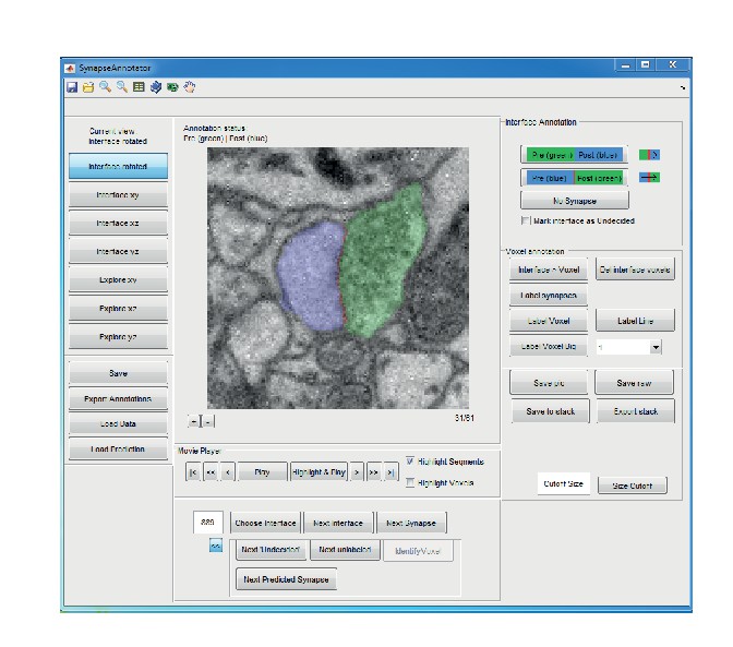
Graphical user interface (implemented in MATLAB) for efficient annotation of neurite interfaces as used for generating the training and validation labels.
3D image data are centered to the neurite interface and rotated such that the second and third principal components of the neurite interface span the displayed image plane. Segments are indicated by transparent overlay (interface, red; subsegment S1, blue and S2, green). Note that the test labels were independently annotated by volume search by multiple experts in webKnossos (Boergens et al., 2017), see Materials and methods.
Figure 3—figure supplement 2
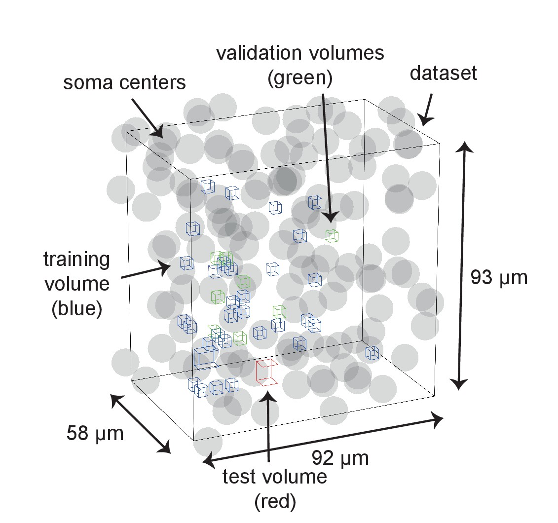
Distribution of training, validation and test data volumes within the dataset 2012-09-28_ex145_07x2.
Soma locations are indicated by spheres of radius 5 μm.
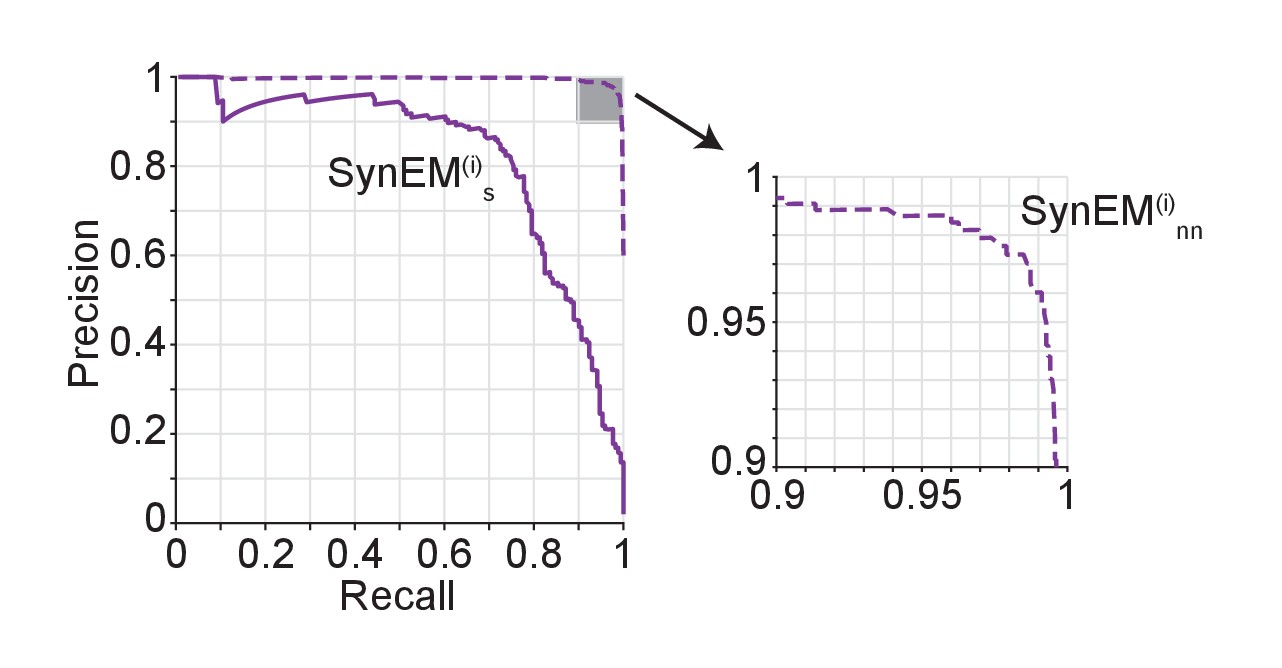
Figure 3—figure supplement 3
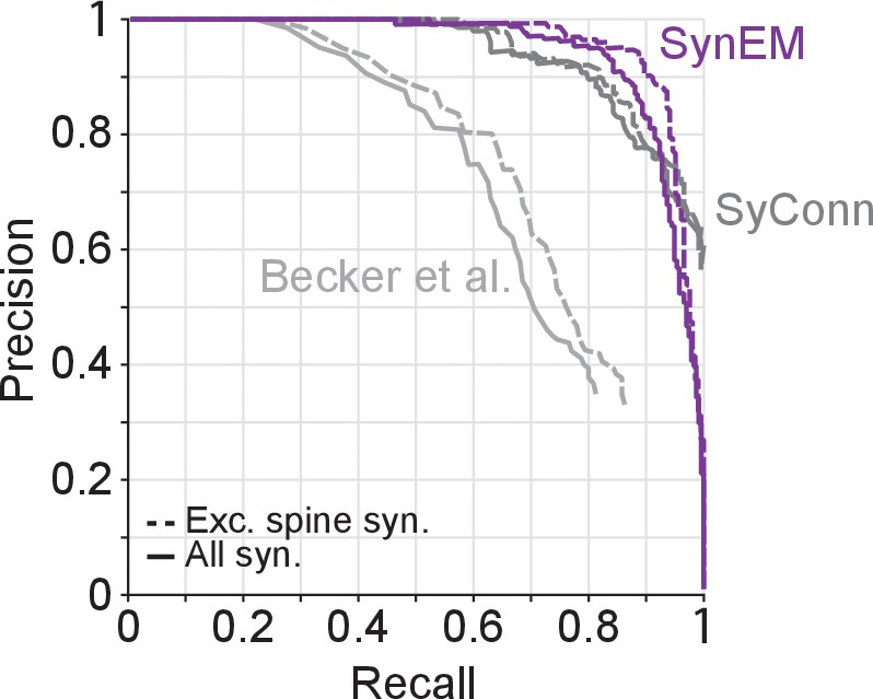
Synapse detection performance comparison of SynEM with SyConn (Dorkenwald et al., 2017) and (Becker et al., 2012) on the 3D SBEM SynEM test set (Figure 3e).
Note that while SynEM performs synapse detection and partner detection in one step these are separate steps in SyConn with an overall performance that is potentially different from the synapse detection step (in Dorkenwald et al., 2017, a reduction in performance by 9% in recall and 2% in precision from synapse detection to partner detection is reported, yielding a drop in F1 score of 0.057). Becker et al. (2012), does not contain a dedicated partner detection step.
-
Figure 3—figure supplement 3—source data 1
- https://doi.org/10.7554/eLife.26414.013
Figure 3—figure supplement 4
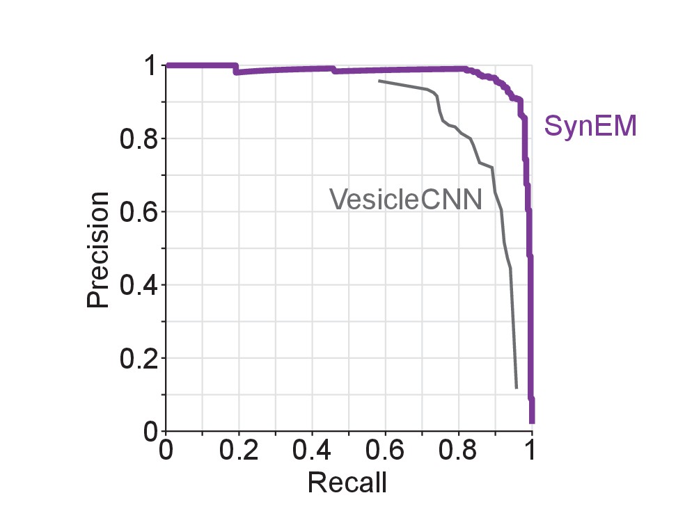
Synapse detection performance comparison of SynEM with VesicleCNN (Roncal et al., 2015) on a 3D EM dataset from mouse S1 cortex obtained using ATUM-SEM (Kasthuri et al., 2015).
Note that VesicleCNN was developed on that ATUM-SEM dataset.
-
Figure 3—figure supplement 4—source data 2
- https://doi.org/10.7554/eLife.26414.015
Figure 4
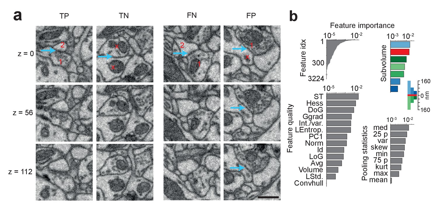
SynEM classification and feature importance.
(a) SynEM classification examples at θs (circle in Figure 3e). True positive (TP), true negative (TN), false negative (FN) and false positive (FP) interface classifications (blue arrow, classified interface) shown as 3 image planes spaced by 56 nm (i.e. every second SBEM data slice, top to bottom). Note that synapse detection in 3D SBEM data requires inspection of typically 10–20 consecutive image slices (see Synapse Gallery in Supplementary file 4 for examples). 1: presynaptic; 2: postsynaptic; x: non-synaptic. Note for the FP example that the axonal bouton (1) innervates a neighboring spine head, but the interface to the neurite under classification (x) is non-synaptic (blue arrow). (b) Ranked classification importance of SynEM features. All features (top left), relevance of feature quality (bottom left), subvolumes (top right) and pooling statistics (bottom right). Note that only 378 features contribute to classification. See Table 2 for the 10 feature instances of highest importance, Table 1 for feature name abbreviations, and text for details. Scale bars, 500 nm.
-
Figure 4—source data 1
Source data for plot in panel 4b.
- https://doi.org/10.7554/eLife.26414.017
Figure 5 with 2 supplements
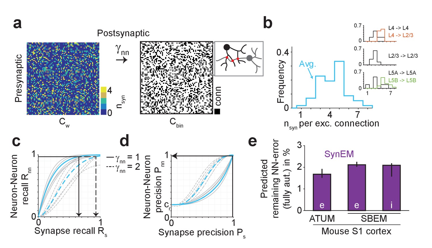
Effect of SynEM classification performance on error rates in automatically mapped binary connectomes.
(a) Sketch of a weighted connectome (left) reporting the number of synapses per neuron-to-neuron connection, transformed into a binary connectome (middle) by considering neuron pairs with at least γnn synapses as connected. (b) Distribution of reported synapse number for connected excitatory neuron pairs obtained from paired recordings in rodent cerebral cortex (Feldmeyer et al., 1999, 2002, 2006; Frick et al., 2008; Markram et al., 1997). Average distribution (cyan) is used for the precision estimates in the following (see Supplementary file 2). (c) Relationship between SynEM recall for single interfaces (synapses) Rs and the ensuing neuron-to-neuron connectome recall Rnn (recall in Cbin, a) for each of the excitatory cortico-cortical connections (summarized in b) and for connectome binarization thresholds of γnn = 1 and γnn = 2 (full and dashed, respectively). (d) Relationship between SynEM precision for single interfaces (synapses) Ps and the ensuing neuron-to-neuron connectome precision Pnn. Colors as in c. (for inhibitory synapses see also Figure 5—figure supplement 1) (e) Predicted remaining error in the binary connectome (reported as 1-F1 score for neuron-to-neuron connections) for fully automated synapse classification using SynEM on 3D EM data from mouse cortex using two different imaging modalities: ATUM-SEM (left, Kasthuri et al., 2015) and our data using SBEM (right). e,i: excitatory or inhibitory connectivity model (see b and Materials and methods) shown for cre = 20% and cri = 60%. Black lines indicate range for varying assumptions of pairwise connectivity rate cre = (5%, 10%, 30%) (excitatory) and cri = (20%, 40%, 80%) (inhibitory). Note that SynEM yields a remaining error of close to or less than 2%, well below expected biological wiring noise, allowing for fully automated synapse detection in large-scale binary connectomes. See Suppl. Figure 5—figure supplement 2 for comparison to previous synapse detection methods.
-
Figure 5—source data 1
Source data for plots in panels 5b, 5c, 5d, 5e.
- https://doi.org/10.7554/eLife.26414.020
Figure 5—figure supplement 1
Performance of SynEM on a test set containing all interfaces between 3 inhibitory axons and all touching neurites (total of 9430 interfaces, 171 synapses).
Single synapse detection precision and recall (solid line) and the ensuing predicted neuron-to-neuron precision and recall for inhibitory connections (dashed line) assuming on average 6 synapses for connections from interneurons (see Materials and methods).
-
Figure 5—figure supplement 1—source data 1
- https://doi.org/10.7554/eLife.26414.022
Figure 5—figure supplement 2
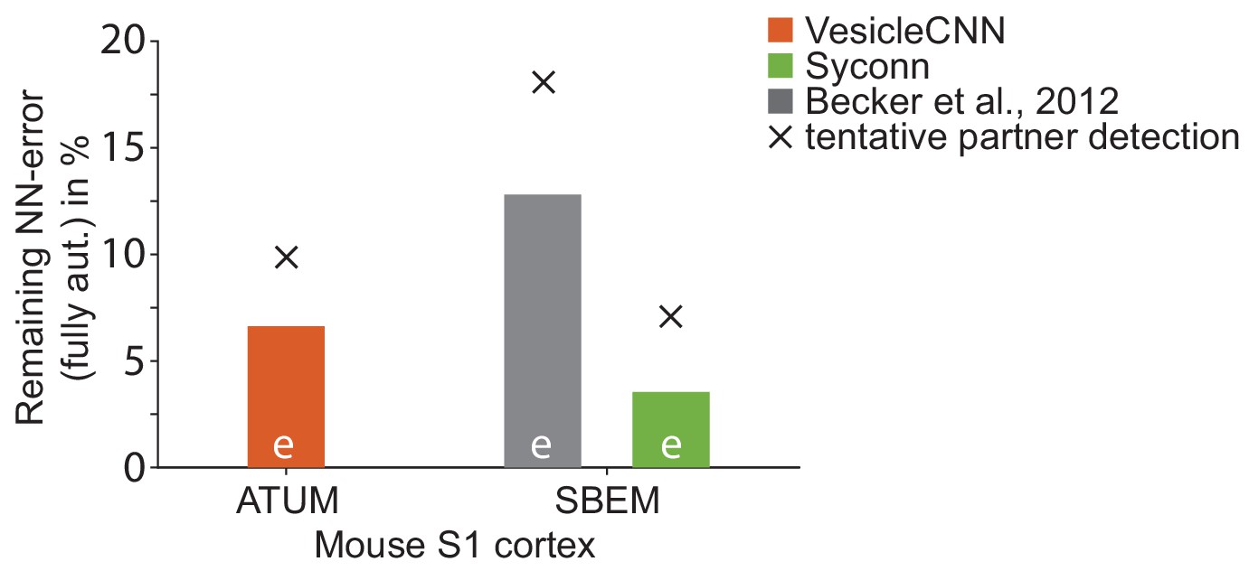
Effect of synapse detection errors on predicted connectome error rates for competing methods.
Predicted neuron-to-neuron errors (reported as (1 F1 score) in percent) for the ATUM-SEM dataset (Kasthuri et al., 2015) using VesicleCNN (Roncal et al., 2015, orange) and for our SBEM dataset using Becker et al. (2012) (gray) and Syconn (Dorkenwald et al., 2017, green). Note that these approaches provide synapse detection, only. When including the detection of the synaptic partners, Dorkenwald et al. (2017) reported a drop of detection performance by 2% precision and 9% recall (indicated by crosses, tentatively also for the other approaches). SynEM provides synapse detection and partner detection together (compare to Figure 5e).
-
Figure 5—figure supplement 2—source data 2
- https://doi.org/10.7554/eLife.26414.024
Figure 6 with 1 supplement
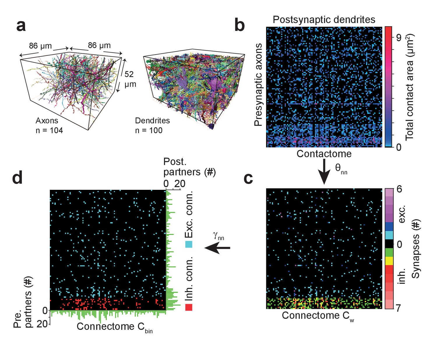
Example sparse local cortical connectome obtained using SynEM.
(a) 104 axonal (94 excitatory, 10 inhibitory) and 100 dendritic processes within a volume sized 86 × 52 × 86 µm3 from layer 4 of mouse cortex skeletonized using webKnossos (Boergens et al., 2017), volume segmented using SegEM (Berning et al., 2015). (b) Contactome reporting total contact area between pre- and postsynaptic processes. (c) Weighted connectome obtained at the SynEM threshold θnn optimized for the respective presynaptic type (excitatory, inhibitory) (see Figure 3e, black square, Table 3). (see also Figure 6—figure supplement 1) (d) Binary connectome obtained from the weighted connectome by thresholding at γnn = 1 for excitatory connections and γnn = 2 for inhibitory connections. The resulting predicted neuron-to-neuron recall and precision were 98%, 98% for excitatory and 98%, 97% for inhibitory connections, respectively (see Figure 5e). Green: number of pre- (right) and postsynaptic (bottom) partners for each neurite.
-
Figure 6—source data 1
Source data for plots in panels 6b, 6c, 6d.
- https://doi.org/10.7554/eLife.26414.026
Figure 6—figure supplement 1
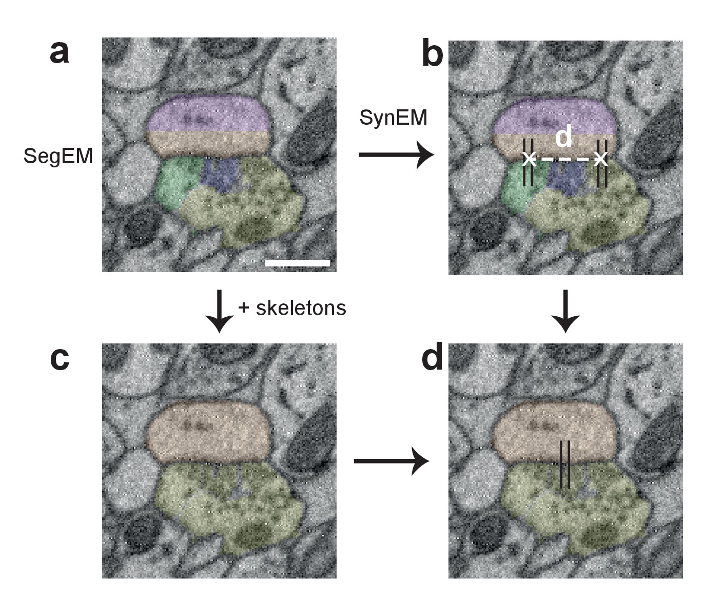
Procedure for obtaining synapse counts in the local connectome (Figure 6).
(a) Segmentation used for SynEM (note that a segmentation biased to neurite splits was used, see Berning et al., 2015) and (b) interfaces detected as synaptic (black lines). (c) combined skeleton-SegEM segmentation of neurites. (d) Synaptic neurite interfaces established between the same pre- and postsynaptic processes (as determined by the skeleton-SegEM segmentation, c) were clustered using hierarchical clustering with a distance cutoff of d = 1.5 μm (b) for obtaining the final synapse count. Scale bar, 500 nm.
Figure 7
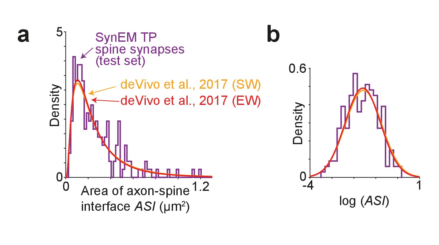
Comparison of synapse size in SBEM data.
(a) Distribution of axon-spine interface area ASI for the SynEM-detected synapses onto spines in the test set from mouse S1 cortex imaged at 11.24 × 11.24 × 28 nm3 voxel size (see Figure 3e), purple; and distributions from de Vivo et al. (2017) in S1 cortex from mice under two wakefulness conditions (SW: spontaneous wake, EW: enforced wake), imaged at higher resolution of 5.9 nm (xy plane) with a section thickness of 54.7 ± 4.8 nm (SW), 51.4 ± 10.3 nm (EW) (de Vivo et al., 2017). (b) Same distributions as in (a) shown on natural logarithmic scale (log ASI SynEM −1.60 ± 0.74, n = 181; log ASI SW −1.56 ± 0.83, n = 839; log ASI EW −1.59 ± 0.81, n = 836; mean ± s.d.). Note that the distributions are indistinguishable (p=0.52 (SynEM vs. SW), p=0.83 (SynEM vs. EW), two-sample two-tailed t-test), indicating that the size distribution of synapses detected in our lower-resolution data is representative, and that SynEM does not have a substantial detection bias towards larger synapses.
-
Figure 7—source data 1
Source data for plots in panels 7a, 7b.
- https://doi.org/10.7554/eLife.26414.030
Author response image 1
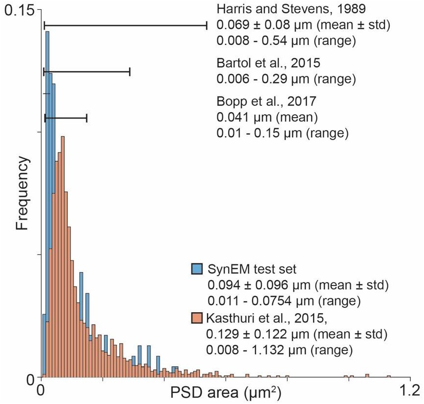
Overview over published PSD area distribution (Harris and Stevens, 1989; Bartol et al., 2015; Kasthuri et al., 2015; Bopp et al., 2017) in comparison to the SynEM test set PSD area distribution.
Ranges as specified in the respective paper (Harris and Stevens, 1989) or estimated from the figures (Bartol et al., 2015; Bopp et al., 2017). The PSD area distribution for (Kasthuri et al., 2015) was calculated using the same method as for the SynEM test set from the synapse segmentation published in (Kasthuri et al., 2015).
Author response image 2
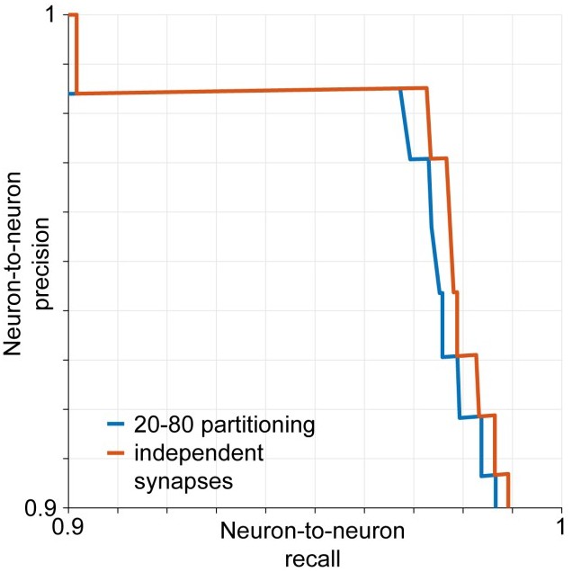
Estimated neuron-to-neuron recall and precision if synapses are assumed to be retrieved independently by the classifier (red) and assuming that 20% of the connections are made exclusively by the 20% smallest synapses and vice versa (blue).
https://doi.org/10.7554/eLife.26414.036Tables
Table 1
Overview of the classifier features used in SynEM, and comparison with existing methods. 11 3-dimensional texture filters employed at various filter parameters given in units of standard deviation (s) of Gaussian filters (s was 12/11.24 voxels in x and y-dimension and 12/28 voxels in z-dimension, sizes of filters were set to σ/s*ceil(2*s)). When structuring elements were used, 1axbxc refers to a matrix of size a x b x c filled with ones and r specifies the semi-principal axes of an ellipsoid of length (r, r, r/2) voxels in x, y and z-dimension. All texture features are pooled by 9 summary statistics (quantiles (0.25, 0.5, 0.75, 0, 1), mean, variance, skewness, kurtosis, respectively) over the 7 subvolumes around the neurite interface (see Figure 2b). Shape features were calculated for three of the subvolumes: border (Bo) and the 160 nm distant pre- and postsynaptic volumes (160). Init. Class: initial SynEM classifier (see Figure 3d for performance evaluation). N of instances: number of feature instances per subvolume (n = 7) and aggregate statistic (n = 9). *: Total number of employed features is 63 times reported instances for texture features. For shape features, the reported number is the total number of instances used, together yielding 3224 features total.
| Features | Kreshuk et al. (2011) | Becker et al. (2012) | Init. class. | SynEM | Parameters | N of instances* |
|---|---|---|---|---|---|---|
| Texture: | ||||||
| Raw data | × | × | × | - | 1 | |
| 3 EVs of Structure Tensor | × | × | × | × | (σw, σd) = {(s,s), (s,2s), (2 s,s), (2 s,2s), (3 s,3s)} | 15 |
| 3 EVs of Hessian | × | × | × | × | σ = {s, 2 s, 3 s, 4 s} | 12 |
| Gaussian Smoothing | × | × | × | σ = {s, 2 s, 3 s} | 3 | |
| Difference of Gaussians | × | × | (σ,k) = {(s, 1.5), (s, 2), (2 s, 1.5), (2 s, 2), (3 s, 1.5)} | 5 | ||
| Laplacian of Gaussian | × | × | × | × | σ = {s, 2 s, 3 s, 4 s} | 4 |
| Gauss Gradient Magn. | × | × | × | × | σ = {s, 2 s, 3 s, 4 s, 5 s} | 5 |
| Local standard deviation | × | U = 15x5x5 | 1 | |||
| Int./var. | × | U = {13x3x3, 15x5x5} | 2 | |||
| Local entropy | × | U = 15x5x5 | 1 | |||
| Sphere average | × | r = {3, 6} | 2 | |||
| Shape: | ||||||
| Number of voxels | × | × | Bo, 160 | 3 | ||
| Diameter (vx based) | × | Bo | 1 | |||
| Lengths of principal axes | × | Bo | 3 | |||
| Principal axis product | × | 160 | 1 | |||
| Convex hull (vx based) | × | Bo, 160 | 3 |
Table 2
SynEM features ranked by ensemble predictor importance. See Figure 4b and Materials and methods for details. Note that two of the newly introduced features and one of the shape features had high classification relevance (Local entropy, Int./var., Principal axes length; cf. Table 1).
| Rank | Feature | Parameters | Subvolume | Aggregate statistic |
|---|---|---|---|---|
| 1 | EVs of Struct. Tensor (largest) | σw = 2s, σD = s | 160 nm, S1 | Median |
| 2 | EVs of Struct. Tensor (smallest) | σw = 2s, σD = s | 160 nm, S1 | Median |
| 3 | Local entropy | U = 15x5x5 | 160 nm, S2 | Variance |
| 4 | Difference of Gaussians | σ = 3 s, k = 1.5 | Border | 25th perc |
| 5 | Difference of Gaussians | σ = 2 s, k = 1.5 | Border | Median |
| 6 | EVs of Struct. Tensor (middle) | σw = 2s, σD = s | 40 nm, S2 | Min |
| 7 | Int./var. | U = 13x3x3 | Border | 75th perc |
| 8 | EVs of Struct. Tensor (largest) | σw = 2s, σD = s | 80 nm, S1 | 25th perc |
| 9 | Gauss gradient magnitude | σ = s | 40 nm, S2 | 25th perc |
| 10 | Principal axes length (2nd) | - | Border | - |
Table 3
SynEM score thresholds and associated precision and recall. SynEM score thresholds θ chosen for optimized single synapse detection (θs) and optimized neuron-to-neuron connection detection (θnn) with respective single synapse precision (Ps) and recall (Rs) and estimated neuron-to-neuron precision and recall rates (Pnn, Rnn, respectively) for connectome binarization thresholds of γnn = 1 and γnn = 2 (see Figure 5).
| Threshold score | Single synapse Ps/Rs | Neuron-to-neuron Pnn/Rnn | |
|---|---|---|---|
| γnn = 1 | γnn = 2 | ||
| θs = -1.67 (exc) | 88.5%/88.1% | 72.5%/99.7% | 98.1%/95.6% |
| θnn = - 0.08 (exc) | 99.4%/65.1% | 98.5%/97.1% | 100%/83.4% |
| θs = -2.06 (inh) | 82.1%/74.9% | 77.1%/100% | 92.7%/99.5% |
| θnn = -1.58 (inh) | 88.6%/67.8% | 84.7%/99.9% | 97.3%/98.5% |
Additional files
-
Supplementary file 1
(Table ) 1 Overview of methods for automated synapse detection.
Res. Fac: Image voxel volume of SBEM data used in this study relative to the voxel volume in the reported studies. Note that most studies employ data of substantially higher image resolution.
- https://doi.org/10.7554/eLife.26414.031
-
Supplementary file 2
(Table) 2 Number of synapses between connected neurons obtained from published studies of paired recordings of excitatory neurons in rodent cortex.
These distributions were used in Figure 5 for prediction of connectome precision and recall.
- https://doi.org/10.7554/eLife.26414.032
-
Supplementary file 3
(Table) 3 Number of synapses between connected neurons obtained from published studies of paired recordings of inhibitory neurons in rodent cortex.
- https://doi.org/10.7554/eLife.26414.033
-
Supplementary file 4
Synapse gallery.
Document describing the criteria by which synapses in 3D SBEM data were detected by human expert annotators. These criteria are exemplified for synapses from the test set of the SynEM classifier.
- https://doi.org/10.7554/eLife.26414.034
Download links
A two-part list of links to download the article, or parts of the article, in various formats.
Downloads (link to download the article as PDF)
Open citations (links to open the citations from this article in various online reference manager services)
Cite this article (links to download the citations from this article in formats compatible with various reference manager tools)
SynEM, automated synapse detection for connectomics
eLife 6:e26414.
https://doi.org/10.7554/eLife.26414


