Microfluidic-based mini-metagenomics enables discovery of novel microbial lineages from complex environmental samples
- Stanford University, United States
- MIT Department of Biological Engineering and Broad Institute of Harvard and MIT, United States
- Department of Energy Joint Genome Institute, United States
- Chan Zuckerberg Biohub, United States
Figures
Figure 1 with 3 supplements
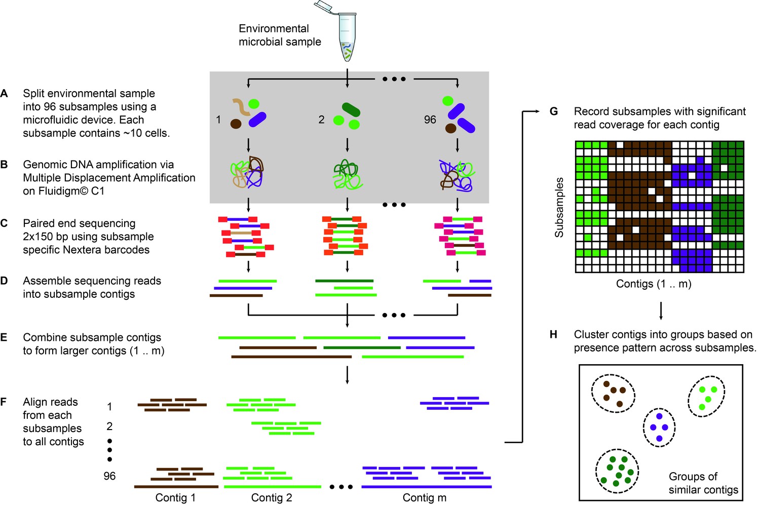
Microfluidic-based mini-metagenomics pipeline.
(A) An environmental microbial sample is loaded onto a Fluidigm C1 IFC at the appropriate concentration so that cells are randomly dispersed into 96 microfluidic chambers at 5–10 cells per chamber. (B) Lysis and MDA are performed on the microfluidic device to generate 1–100 ng genomic DNA per sub-sample. (C) Nextera libraries are prepared from the amplified DNA off-chip and sequenced using 2 × 150 bp runs on the Illumina NextSeq platform. (D) Sequencing reads from each sub-sample are first assembled independently, then (E) sub-sample contigs are combined to form longer mini-metagenomic contigs. Contigs longer than 10 kbp are processed in the following steps. (F) Reads from each sub-sample are aligned to mini-metagenomic contigs > 10 kbp. (G) An occurrence map is generated, demonstrating the presence pattern of each contig in all sub-samples based on coverage. (H) Finally, contigs are binned into genome clusters based on a pairwise p value generated from co-occurrence information. Steps enclosed in the gray rectangle (A, B) are performed on the Fluidigm C1 IFC. Step C is carried out in 96 well plates. Steps D to H are performed in silico.
Figure 1—figure supplement 1
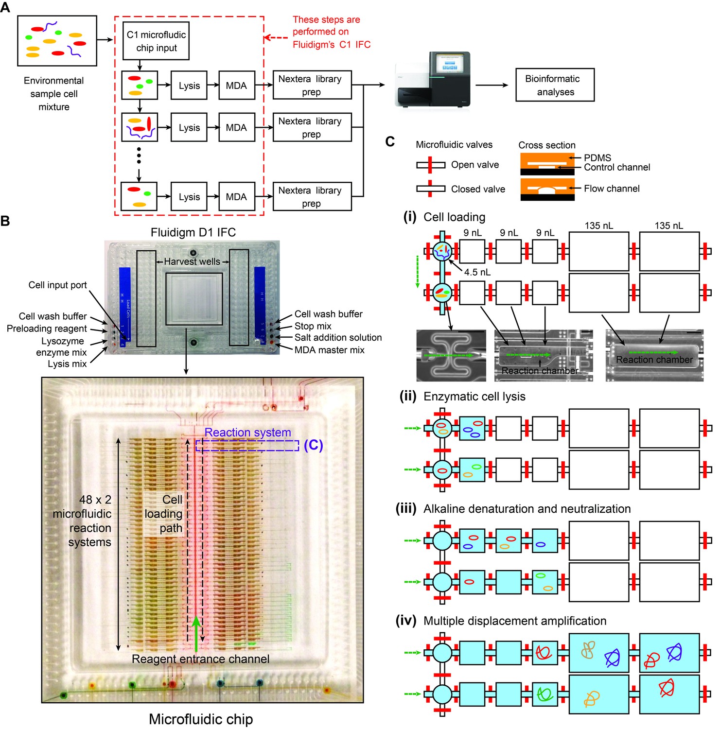
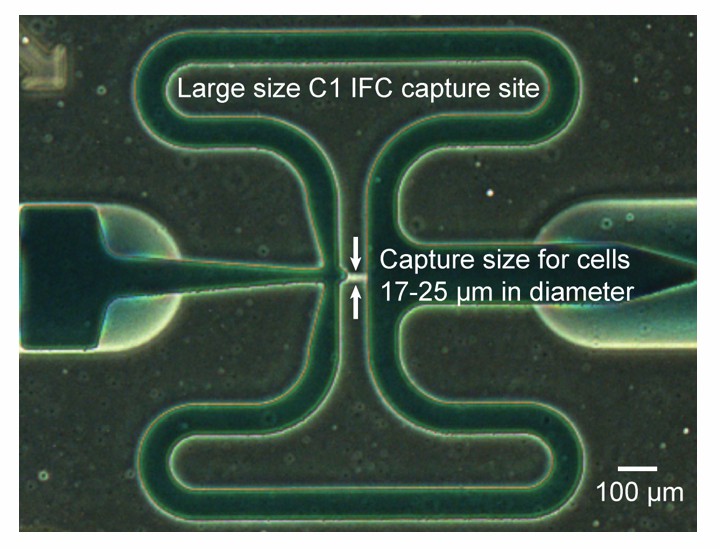
Details of the mini-metagenomic experimental steps performed on the Fluidigm C1 microfluidic IFC.
(A) Cells are distributed randomly into 96 chambers with no size selection. Enzymatic lysis, DNA denaturation, and whole genome amplification via MDA (Multiple Displacement Amplification) occurs on chip. Amplified DNA is harvested for off-chip library preparations, sequencing, and bioinformatic analyses. (B) Image of a Fluidigm C1 IFC. The polydimethylsiloxane (PDMS) chip is located in the center of a plastic cartridge, which contains wells for inputting cells, reagents, and for harvesting amplified genomic DNA. The cartridge has the dimensions of a standard cell culture plate. Below the image of the C1 IFC, the PDMS microfluidic chip located in the center of the plastic cartridge is enlarged and partially filled with food coloring to illustrate high level organizations of the microfluidic circuit. Each chip contains 96 independent reaction systems split into a mirrored 48 × 2 array, extending from the center channel (filled with red food coloring) to the left and right edges of the chip. The cell loading path (dashed black arrow) and reagent entrance channel (solid green arrow) are denoted. (C) Each reaction system contains one capture chamber and five sequential reaction chambers with different sizes. The first 3 reaction chambers of all reactions systems are filled with food coloring in (B). Two adjacent reaction systems (dashed purple lines in (B) are selected to demonstrate their functions. Red bars represent microfluidic valves whose open and closed states are shown through their cross sections. Green arrows represent flow directions of reagents. All reaction chambers are initially empty (i.e. filled with air). (i) During cell loading, capture chambers are connected and cells are randomly distributed across all capture chambers. Following cell loading, all reaction systems are isolated via valves. Sample images of the microfluidic chambers are shown (black scale bars represent 200 μm). Sequential reactions of (ii) enzymatic lysis to release DNA, (iii) alkaline denaturation and neutralization, and (iii) MDA to amplify DNA are carried out by filling additional empty chambers with reagents. Amplified DNA is flushed into harvest wells for extraction and subsequent off-chip steps.
Figure 1—figure supplement 2
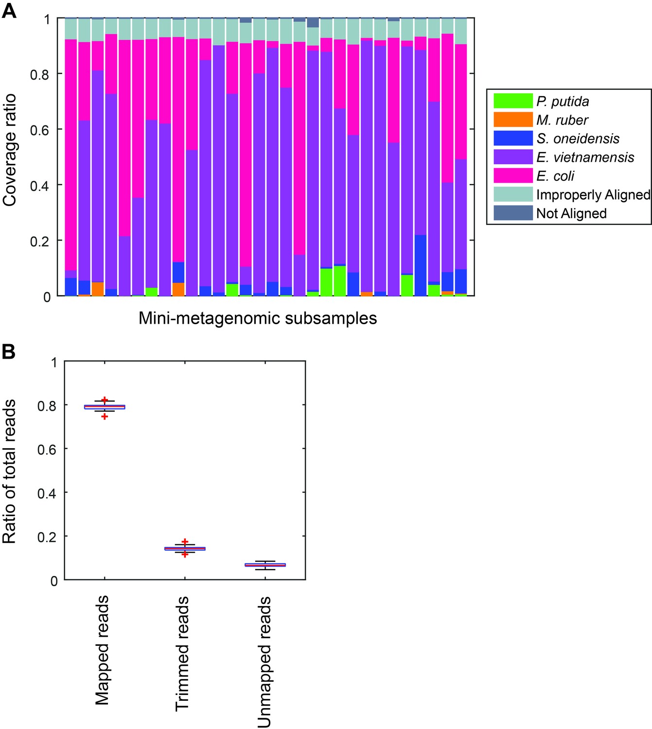
Performance of microfluidic-based mini-metagenomic amplification.
A mock community is constructed and processed using the microfluidic-based mini-metagenomic pipeline. (A) Reads from each subsample are mapped back to known reference genomes. Over 90% of reads map uniquely to one of the five species. Improperly aligned reads are typically reads of poor sequencing quality or are too short to have good alignment scores. Less than 2% are unmapped. (B) Typically, 15% of raw sequencing reads are trimmed based on quality scores. 5% reads are unmapped or improperly mapped, mostly represented by short library fragments. Less than 1% are chimeric reads.
Figure 1—figure supplement 3
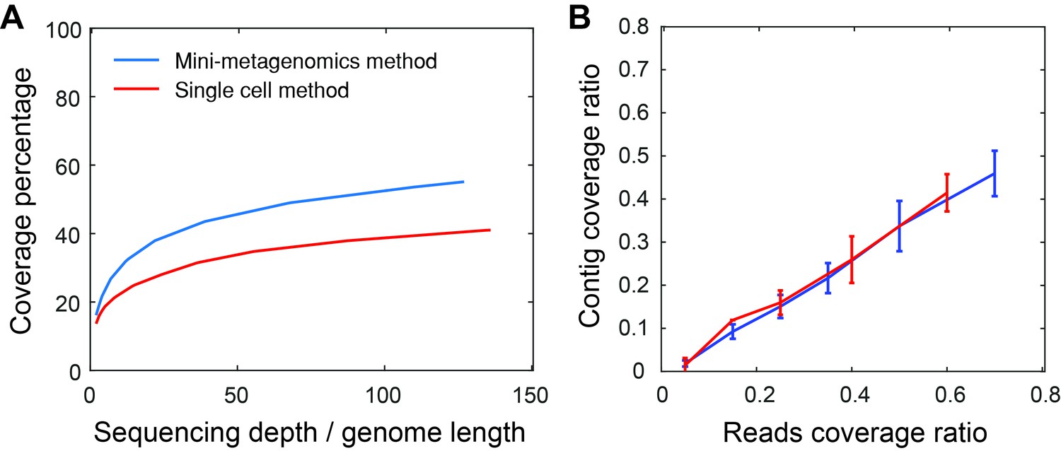
Mini-metagenomics performance on mock communities.
(A) Compared to the single-cell method, mini-metagenomics showed a superior rarefaction curve. The percent genome coverage recovered from the mini-metagenomic method was higher than using single-cell metagenomic methods for all sequencing depths. (B) Given a particular read coverage percentage, both mini-metagenomic and single-cell methods yielded similar contig coverage ratios.
Figure 2 with 6 supplements
Genome bins extracted from microfluidic-based mini-metagenomic sequencing of Yellowstone National Park samples.
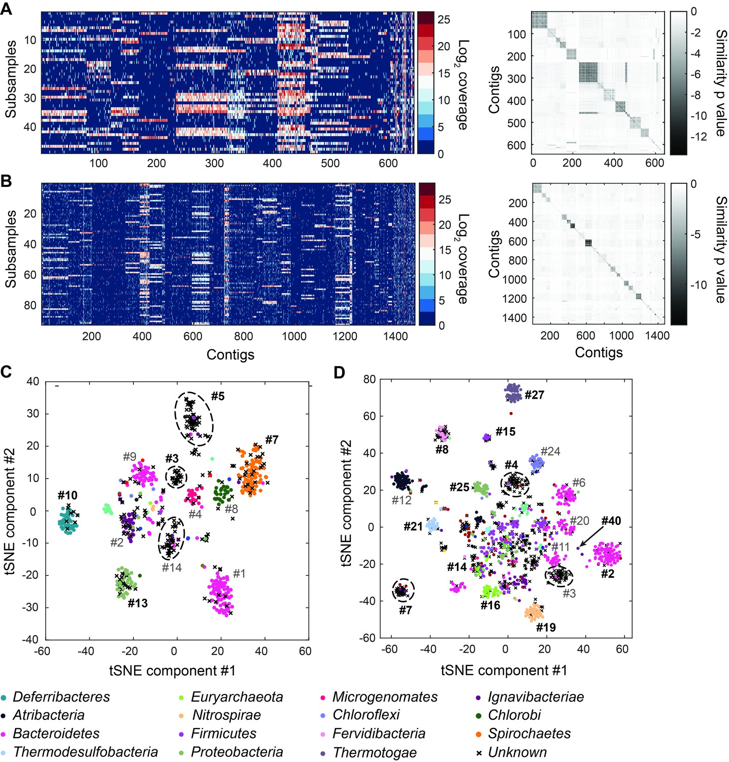
Two samples from Bijah Spring in Mammoth Norris Corridor (A, C) and Mound Spring in Lower Geyser Spring Basin (B, D) were collected from Yellowstone National Park and analyzed using the microfluidic-based mini-metagenomic pipeline. (A, B) Heat maps of contig coverage across sub-samples are clustered hierarchically to reveal contigs that appear in similar sets of sub-samples (left). Colors represent logarithm of coverage in terms of number of base pairs in base 2. Pairwise p values generated using Fisher’s exact test based on co-occurrence pattern of contig pairs reveal contig clusters (right). Shading here represents logarithm of p value in base 10 after correcting for multiple comparisons. (C, D) tSNE dimensionality reduction generated from pairwise p values. Each point represents a 10 kbp or longer contig. Colors represent assignment of each contig to a particular phylum based on annotation of genes on the contig. Black X’s represent contigs unable to be assigned to any phylum because too many genes have unknown annotation. Genome bins larger than 0.5 Mbp are numbered and those with substantial numbers of single-copy marker genes for incorporation into Figure 4 are labeled in bold. Dotted circles outline genomes predominantly containing contigs unassigned at the phylum level.
Figure 2—figure supplement 1
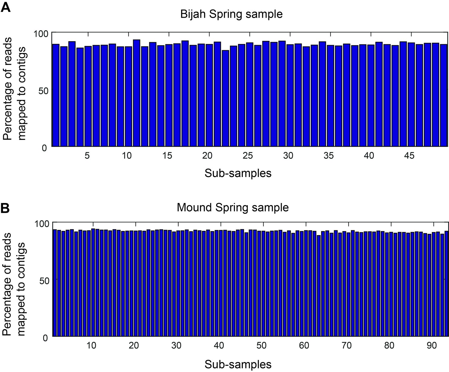
Mapping rate of mini-metagenomic sequences.
Approximately 90% of the reads were routinely incorporated into contigs 1 kbp or greater in every sub-sample for (A) Bijah and (B) Mound Spring samples.
Figure 2—figure supplement 2
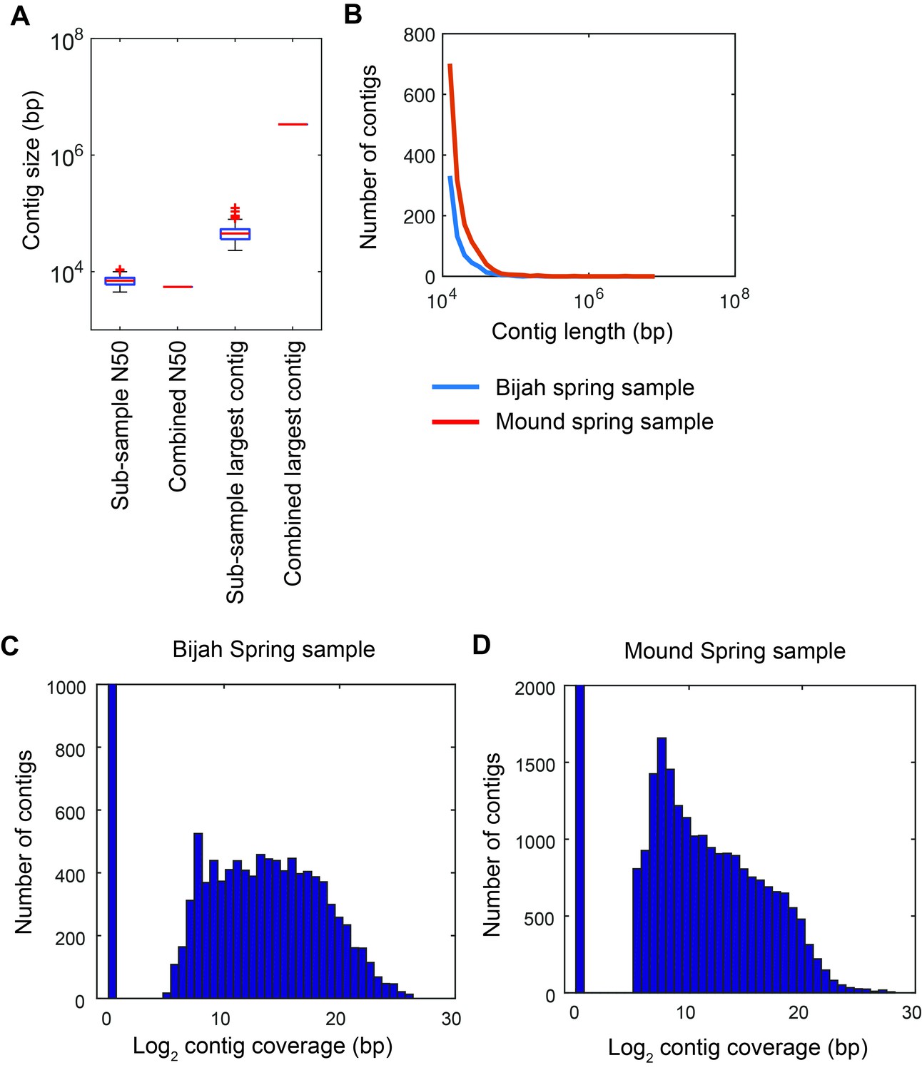
Contig statistics of Yellowstone National Park samples.
(A) Sub-sample N50 and largest contig size in comparison with N50 and largest contig size for the combined assembly of all sub-samples reads. Assessment was done on contigs longer than 500 bps. Plot represents Mound Spring statistics. (B) Distribution of contig lengths for samples from Bijah (blue) and Mound (red) Springs. Plot shows only contigs greater than 10 kbp. Histogram of covered contig length from reads belonging to every sub-sample in (C) Bijah Spring and (D) Mound Spring samples. Coverage of 211 bps was required for a contig to be designated as present in a sub-sample.
Figure 2—figure supplement 3
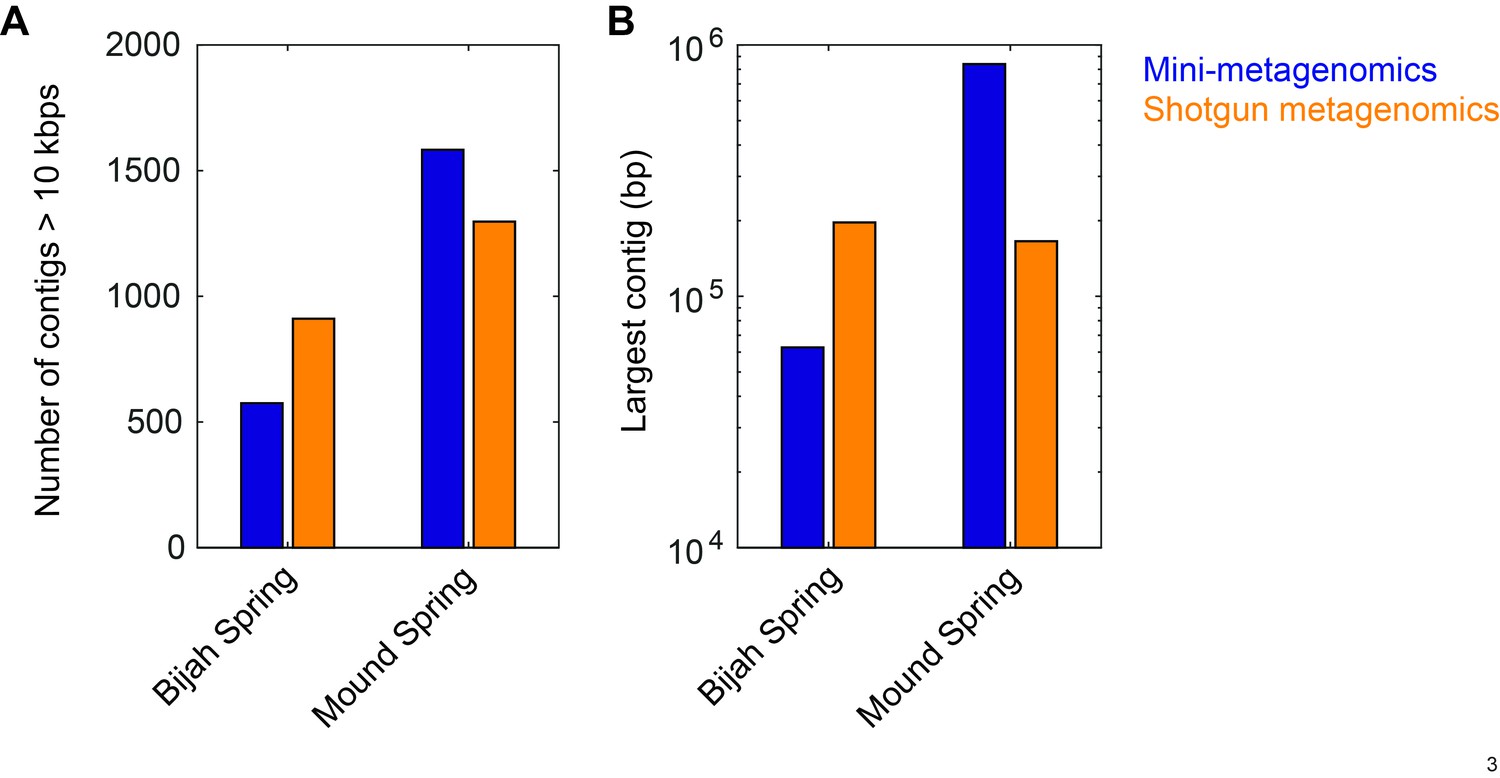
Comparison between contig statistics of mini-metagenomic and shotgun metagenomic assemblies.
Mini-metagenomic reads from all subsamples (49 for Bijah Spring and 93 for Mound Spring) were combined and randomly subsampled to the same depth as shotgun metagenomic sequencing depth of 32.5 million and 51.4 million reads, respectively. Mini-metagenomic reads were assembled using SPAdes (Bankevich et al., 2012) while Shotgun metagenomic reads were assembled using Megahit (Li et al., 2015). Contigs over 10 kbps were tabulated using Quast (Gurevich et al., 2013). (A) Number of contigs over 10 kbps showing that shotgun metagenomics generated more contigs over 10 kbps in the Bijah Spring sample but less contigs in Mound Spring sample compared to mini-metagenomic assemblies. (B) Largest contig from shotgun metagenomic assembly was longer than the largest mini-metagenomic contig in the Bijah Spring sample but was shorter in the Mound Spring sample.
Figure 2—figure supplement 4
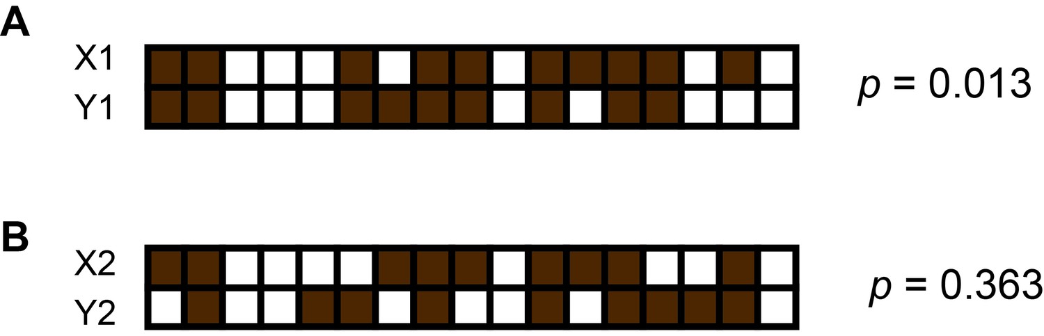
An example of computing p values using Fisher’s exact test and presence patterns of two contigs.
Here, brown squares represent sub-samples in which the contig is present and white squares represent those from which the contig is missing. The computed p value using the equation. Where. a = number of sub-samples where X is present and Y is present. b = number of sub-samples where X is absent and Y is present. c = number of sub-samples where X is present and Y is absent. d = number of sub-samples where X is absent and Y is absent. p represents the probability of incorrectly rejecting the null hypothesis that presence patterns of the two contigs X and Y occur randomly. (A) Presence patterns of X1 and Y1 are correlated because we obtain a small p. (B) We cannot reject the null hypothesis here due to the large p obtained.
Figure 2—figure supplement 5
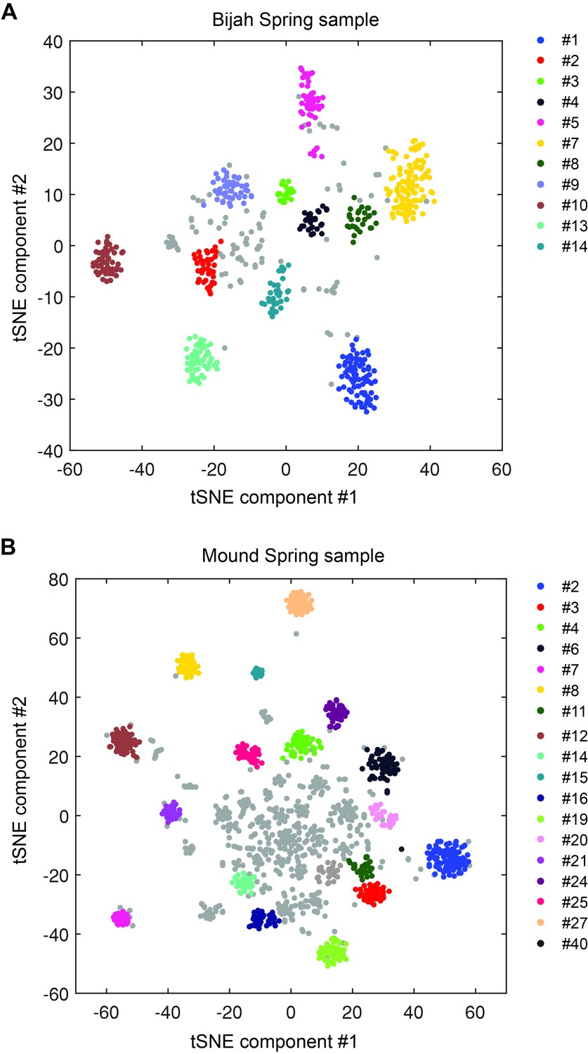
DBscan clustering of mini-metagenomic contigs.
Cluster results applying DBscan to the output of tSNE dimensional reduction based on pairwise p value matrix. Plots represent (A) Bijah Spring and (B) Mound Spring samples. Cluster numbers correspond to labels in Figure 2C,D. Gray contigs represent those that were not incorporated into a large enough contig cluster.
Figure 2—figure supplement 6
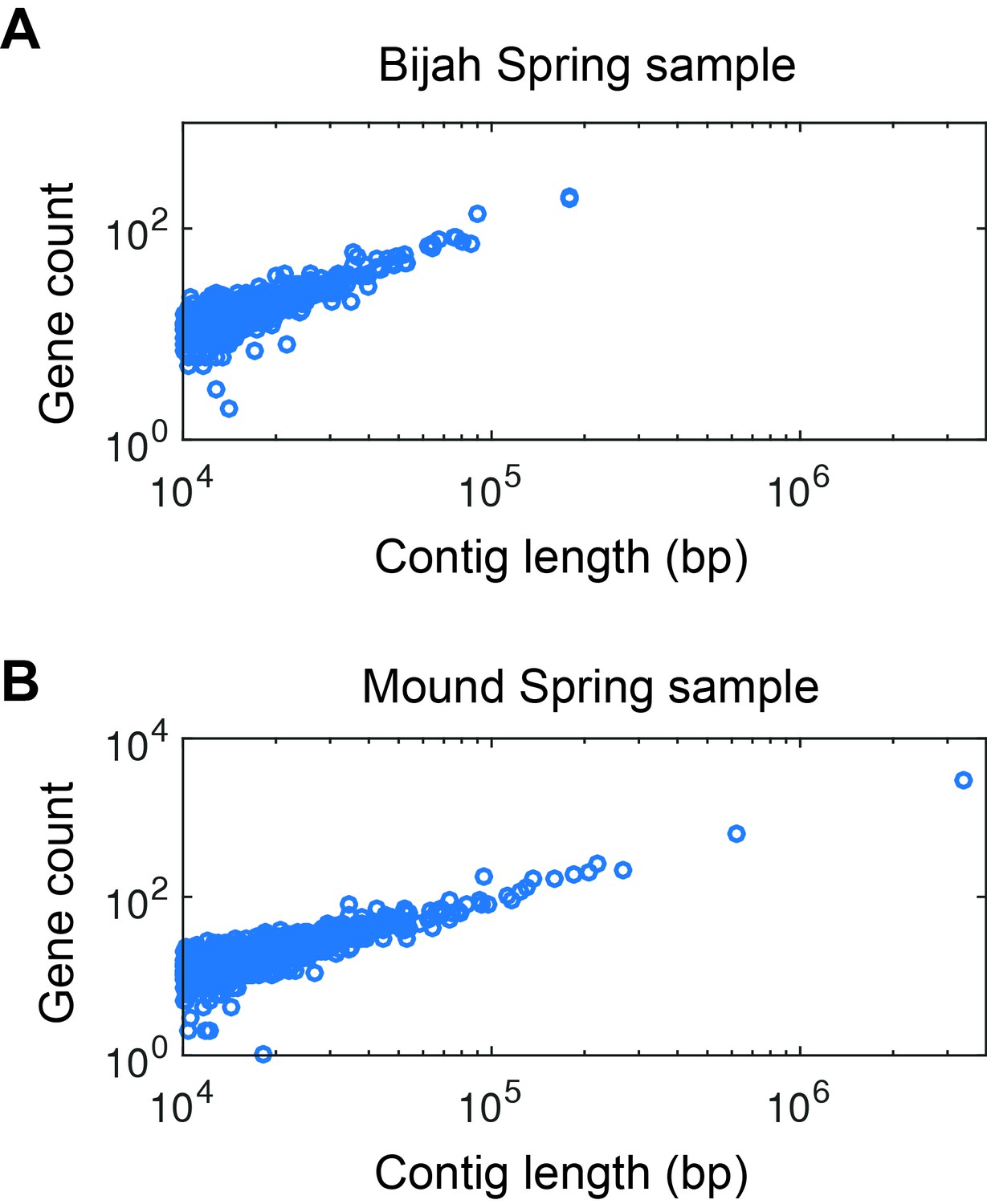
Gene count as a function of contig length.
Gene count as a function of contig length for (A) Bijah and (B) Mound Spring samples. Only contigs larger than 10 kbp are shown. The linear relationship is consistent with little non-coding regions in bacterial genomes, increasing the likelihood that these contigs represent biological entities instead of sequencing artifacts.
Figure 3
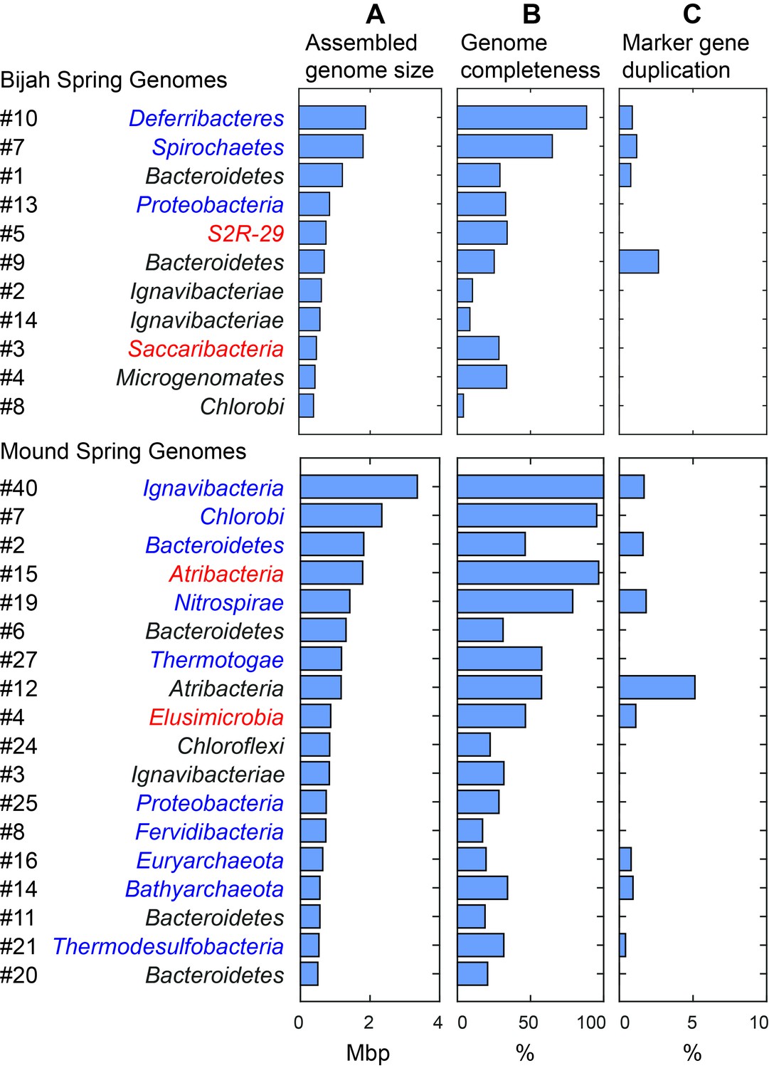
Assembled size and completeness of Yellowstone hot spring genomes.
Genomes of Bijah Spring and Mound Spring samples are sorted by assembled genome size (A). Names represent phylum level assignment based on annotated genes (Figure 2), concatenated marker gene phylogenetic tree (Figure 4), or individual marker gene trees (Figure 4—figure supplement 1, Figure 4—figure supplement 2). (B) Genome completeness is assessed through single-copy marker genes; those incorporated into Figure 4 have phyla names colored in blue (for short branching lineages) or red (for deeply branching lineages). (C) Degree of marker gene duplication in assembled genomes assessed using CheckM (Parks et al., 2015).
Figure 4 with 2 supplements

Phylogenetic distribution of selected Yellowstone hot spring genomes (red branches) across a representative set of bacterial and archaeal lineages.
Query genomes which potentially represent novel phyla are marked with a star, and those falling into known phyla are highlighted in yellow. Bootstrap support values are displayed at the nodes as filled circles in the following categories: no support (black; <50), weak support (grey; 50–70), moderate support (white; 70–90), while absence of circles indicates strong support (>90 bootstrap support). For details on taxon sampling and tree inference, see Materials and methods.
Figure 4—figure supplement 1
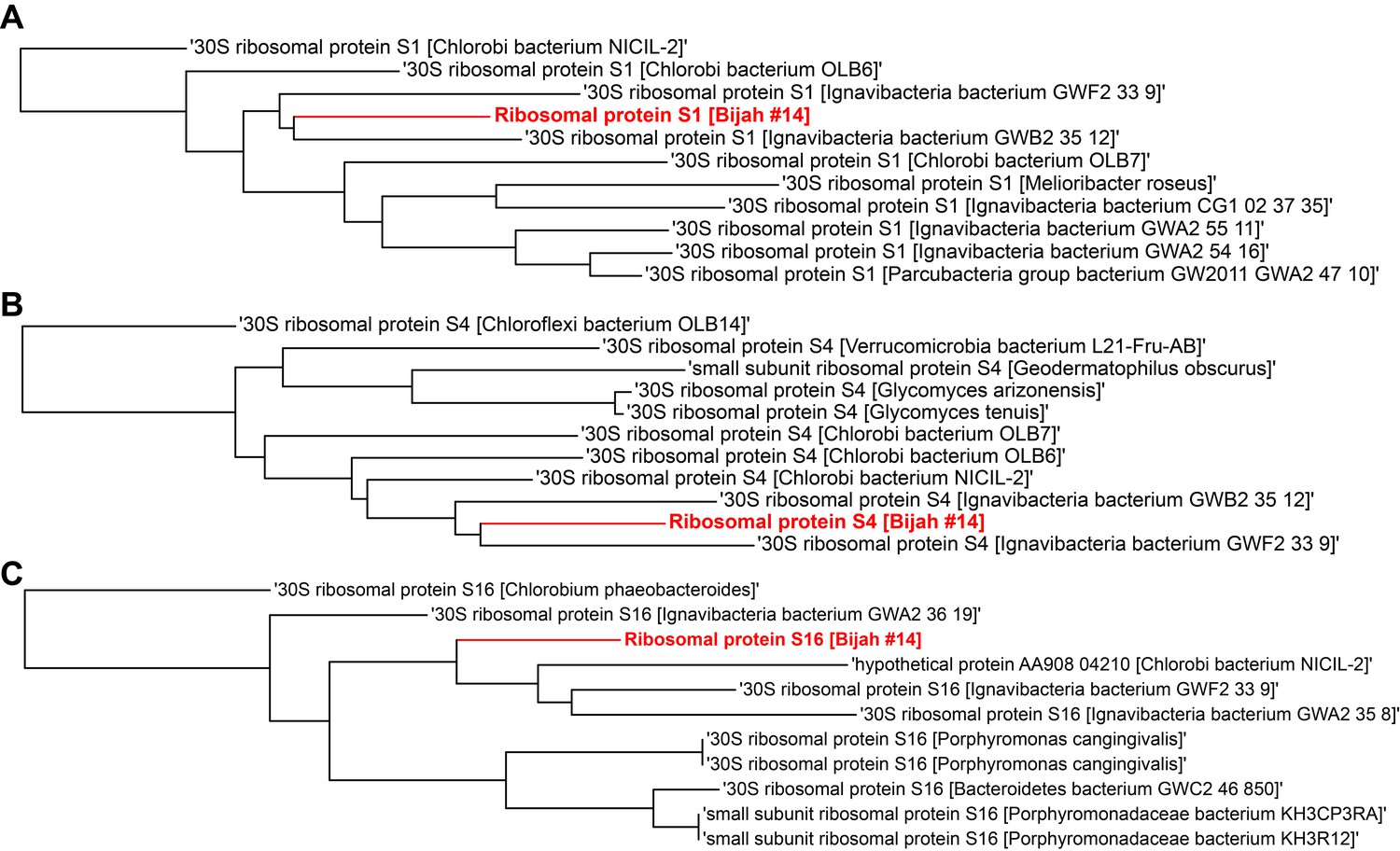
Single gene trees based on multiple sequence alignment of 10 most similar protein sequences for Bijah Spring genome #14 based on NCBI protein blast.
Three longest ribosomal protein sequences identified in the genome were used including (A) ribosomal protein S1, (B) ribosomal protein S4, (C) ribosomal protein S16.
Figure 4—figure supplement 2
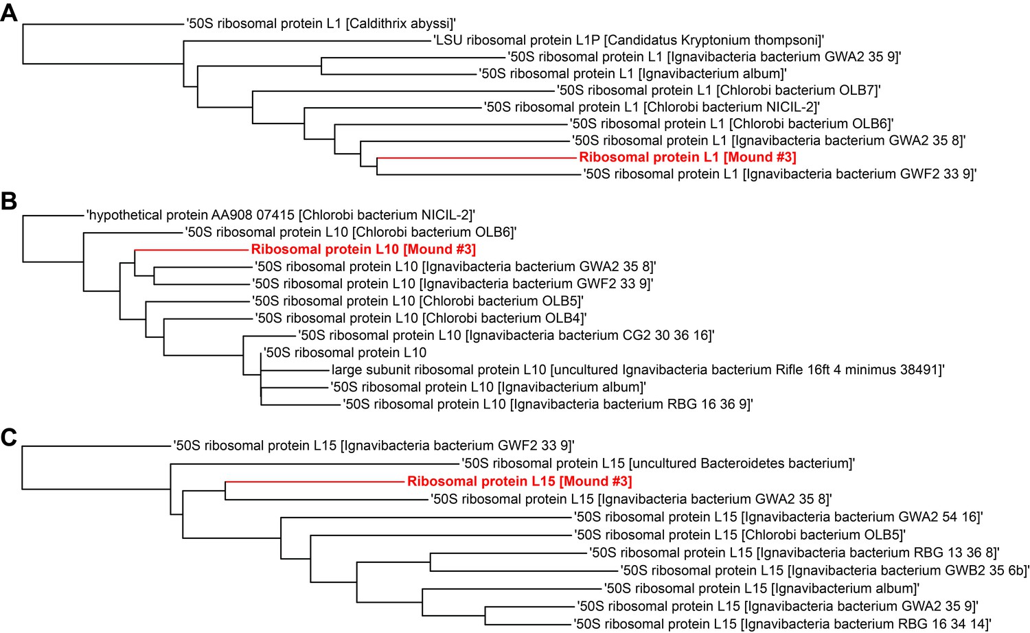
Single gene trees based on multiple sequence alignment of 10 most similar protein sequences for Mound Spring genome #3 based on NCBI protein blast.
Three longest ribosomal protein sequences identified in the genome were used including (A) ribosomal protein L1, (B) ribosomal protein L10, (C) ribosomal protein L15.
Figure 5
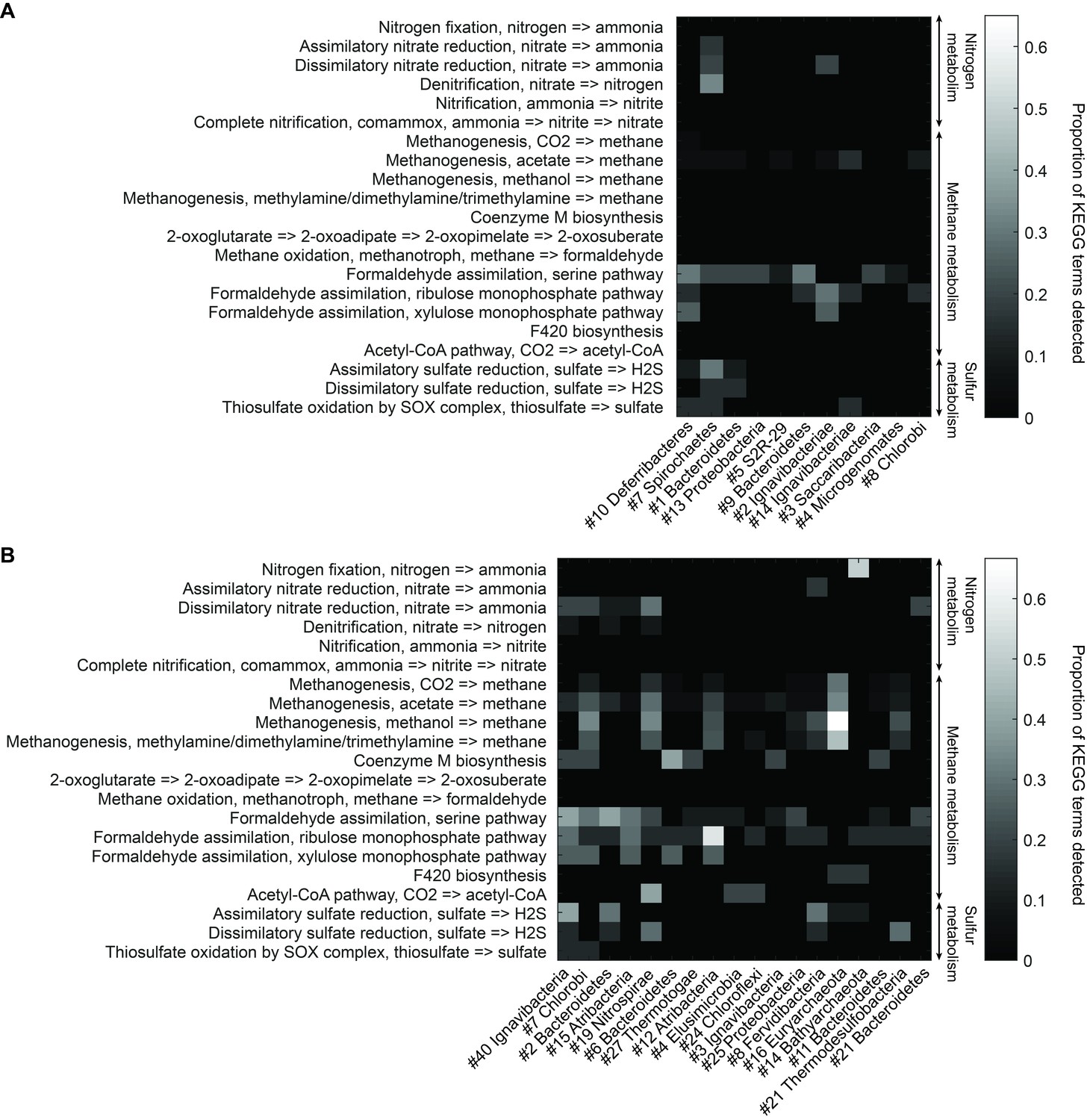
Functional analysis of Yellowstone hot spring genomes.
Abundant genes involved in energy metabolism of (A) Bijah Spring and (B) Mound Spring genomes. Each row represents description of a pathway based on KEGG energy metabolism modules. Each column represents one genome bin. Shading of each square represents the ratio of genes in each KEGG module that are also present in a particular genome bin. Modules are labeled as nitrogen metabolism, methane metabolism, or sulfur metabolism.
Figure 6 with 2 supplements
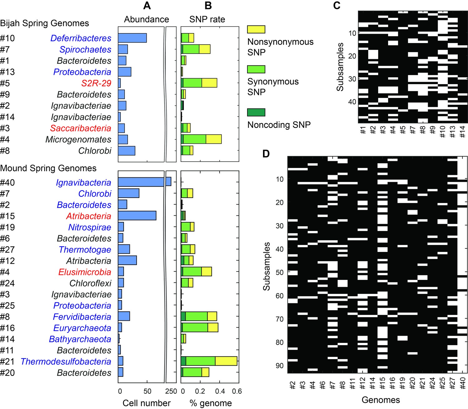
Abundance and population variation of Yellowstone hot spring genomes.
(A) Abundance is derived from the occurrence pattern of contig clusters, where Poisson distribution is used to infer the number of cells processed. (B) SNPs are tabulated and normalized by the total size of sequenced genome. Most SNPs are in coding regions of the genome, of which the majority are synonymous. (C, D) Map of genome occurrence patterns across all sub-samples for (C) Bijah and (D) Mound Springs samples. White demonstrates the presence of at least one cell of a particular genome in a sub-sample. The total number of cells can be inferred using Poisson statistics.
Figure 6—figure supplement 1
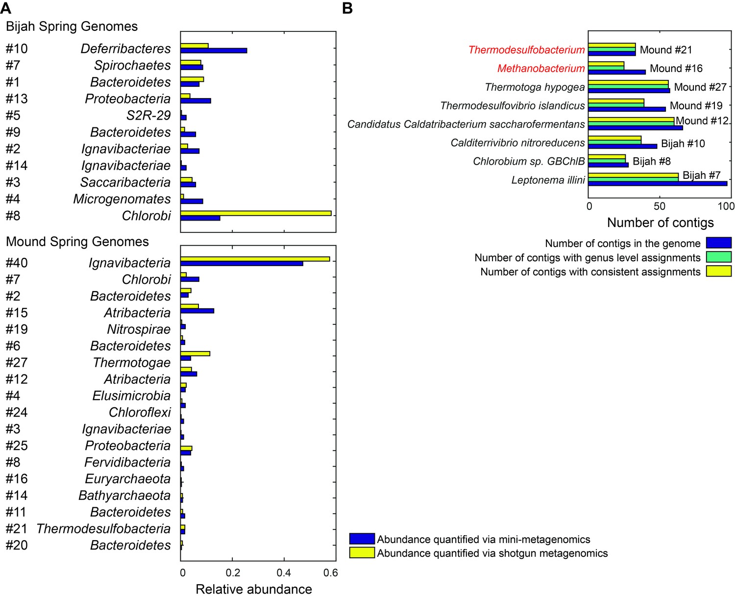
Genome relative abundance and taxonomic specificity.
(A) Comparison between genome abundance computed using mini-metagenomics and shotgun metagenomics. Shotgun metagenomic abundance was computed by counting the number of shotgun reads mapped to genomes generated using mini-metagenomics. Mapping was accomplished using bowtie2 with options --very-sensitive -I 100 -X 2000. Abundance profiles were normalized by either the total number of cells or the total number of reads, yielding a measure of relative abundance. (B) Taxonomic specificity of selected genomes. Six genomes with more than 50% of the contigs having phylogenetic lineage assignments at the species level were selected from both springs (black). The plot displays the number of contigs in the genome (dark blue), the number of contigs with genus level assignments (green), and the number of contigs assigned to the species shown on the left of the plot (yellow). Almost all contigs in a genome were assigned to the same species. Two genomes (red) had high levels of specificity at genus level assignments but were predominantly unassigned at the species level: Methanobacterium and Thermodesulfobacterium. These genomes represented novel species in respective genera.
Figure 6—figure supplement 2
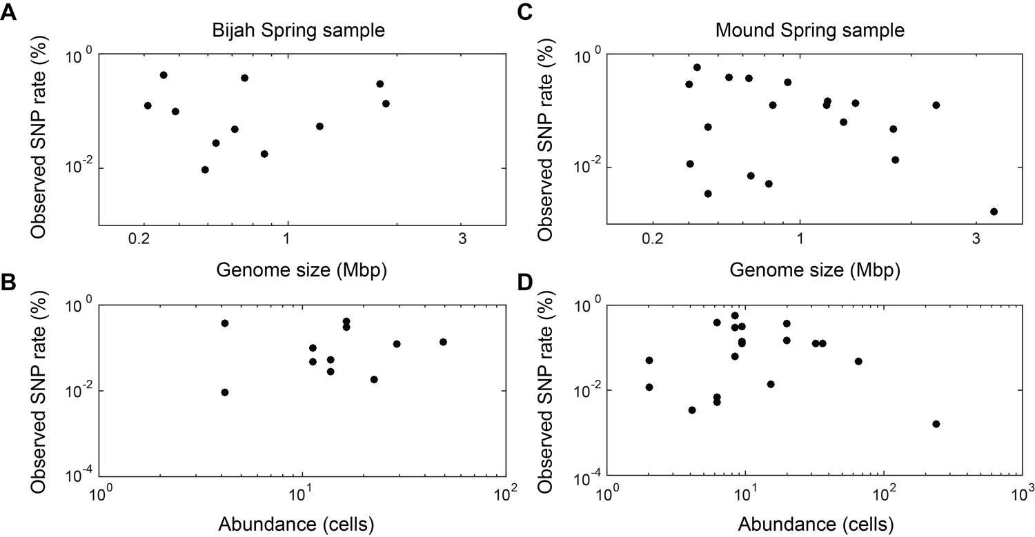
Observed SNP rates compared to other variables.
Observed SNP rates as a function of (A, C) genome size and (B, D) genome abundance for all genomes in (A, B) Bijah and (C, D) Mound Springs samples. SNP rate was quantified by summing all observed SNPs for a particular genome in all cells and normalizing to the total length of DNA sequenced from those cells. There does not seem to be any clear correlations between SNP rate and genome size or abundance.
Author response image 1
Tables
Table 1
Species used to construct mock bacterial communities.
| Species name | GC content (%) | Culture source | Growth medium | Assession numbers |
|---|---|---|---|---|
| Echinicola vietnamensis KMM6221 | 44.7 | DSM 17526 | Marine broth | NC_019904.1 |
| Shewanella oneidensis MR1 | 45.9 | JGI | LB | NC_004347.2 |
| Escherichia coli MG1655 | 50.8 | ATCC 700926 | LB | NC_000913.3 |
| Pseudomonas putida F1 | 61.9 | ATCC 700007 | Nutrient medium | NC_009512.1 |
| Meiothermus ruber | 63.4 | DSM 1279 | Termus ruber medium | NC_013946.1 |
Table 2
Information of hot spring samples from Yellowstone National Park.
| Sample #1 | Sample #2 | |
|---|---|---|
| NPS study number | YELL_05788 | YELL_05788 |
| Sample area | Mammoth Norris Corridor | Lower Geyser Basin |
| Location name | Bijah Spring | Mound Spring |
| Sample type | Sediment | Sediment |
| Collection time | September 11, 2009 5:00pm | September 14, 2009 2:25pm |
| Location | 44.761133 N, 110.730900 W | 44.564833 N, 110.859933 W |
| Location type | Hot spring | Hot spring |
| Temperature (°C) | 65 | 55 |
| pH | 7.0 | 9.0 |
Table 3
Yellowstone sample sequencing and assembly statistics.
| Sample #1 | Sample #2 | |
|---|---|---|
| IMG genome ID | 3300006068 | 3300006065 |
| Number of molecules sequenced | 120.5 M | 133.1 M |
| Number of contigs (>10 kbp) | 643 | 1474 |
| Number of subsamples analyzed | 49 | 93 |
Additional files
-
Supplementary file 1
Table of COG terms used for making marker gene based phylogenetic tree (Figure 4).
- https://doi.org/10.7554/eLife.26580.024
Download links
A two-part list of links to download the article, or parts of the article, in various formats.
Downloads (link to download the article as PDF)
Open citations (links to open the citations from this article in various online reference manager services)
Cite this article (links to download the citations from this article in formats compatible with various reference manager tools)
Microfluidic-based mini-metagenomics enables discovery of novel microbial lineages from complex environmental samples
eLife 6:e26580.
https://doi.org/10.7554/eLife.26580


