A quantitative theory of gamma synchronization in macaque V1
- Maastricht University, Netherlands
- Radboud University Nijmegen, Netherlands
- Ernst Strüngmann Institute (ESI) for Neuroscience in Cooperation with Max Planck Society, Germany
Figures
Figure 1 with 2 supplements
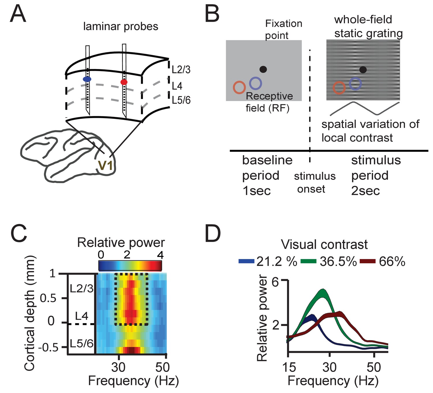
Experimental setup and contrast-dependent V1 gamma frequencies.
(A) Schematic rendering of recording location. Two to three laminar probes were inserted with 1–6 mm separation in cortical area V1. (B) The visual paradigm consisted of a 1 s baseline period with a gray background and 2 s visual stimulation with a full-screen static grating characterized by spatially varying local contrast. During both periods the monkeys maintained their gaze on a fixation point (controlled by eye tracking). For analysis, the stimulation period (0.2–2 s) was used, not including the first 200 ms to avoid stimulus-evoked transients. Two receptive fields (RF) from different probes are shown on the grating stimulus (blue and red circles). The aim was to modulate (detune) the local frequencies of gamma rhythms using local contrast differences. (C) Spectral power relative to baseline as a function of V1 cortical depth (36.5% contrast, population average, M1). Data for gamma analysis are taken from granular and superficial layers (dashed box) unless stated otherwise. (D) Local contrast modulated gamma frequency (population average, M1) as shown in the power spectral profile for three of the five contrast values employed. Width of shaded area represents SE.
Figure 1—figure supplement 1
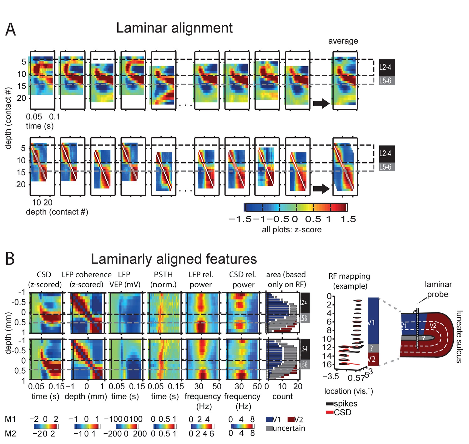
Cortical depth alignment and analysis.
(A) Alignment procedure: CSDs from single sessions and probes were shifted iteratively to minimize the squared error between all probes using a parallel tempering algorithm until an optimal constellation of shifts was reached. Gamma-range coherence was then used to confirm or improve the constellation (see text for details). From left to right: example sessions from the first few and last few recording days, at the very right: average across all sessions, including sessions not shown here. Top row: CSD, bottom row: gamma-range coherence during baseline grey screen period. Black/grey lines indicate location of layers 2–4 versus 5–6. Example sessions are taken from monkey M2. (B) Depth-aligned grand average features per monkey, top row monkey M1, bottom row monkey M2. Black/grey lines indicate location of layers 2–4 versus 5–6. Zero indicates last channel included in L2-4, black/grey lines overlap the reversal point. From left to right: CSD, LFP gamma-band coherence as used for alignment, visual evoked potential, peristimulus time histogram (PSTH), LFP and CSD power in the gamma range, area assignment based on receptive field jumps. The PSTH of each session was normalized to the maximum activity of the maximally active spike channel. Relative power was computed as stimulus/baseline (baseline averaged across trials) for both LFP and CSD. The rightmost column shows the number of contacts assigned to each depth and their assignment to V1 vs. white matter or V2 based on receptive field mapping alone, providing an estimate independent of the CSD reversal point. Grey contacts were either those positioned likely in white matter, just preceding a receptive field jump, or all contacts if no receptive field jump was present (most likely representing all contacts still in V1). An example RF mapping to the right together with a sketch illustrates this procedure. Receptive fields as estimated by spiking (black) and CSD (red) show a clear jump at contact 14, entering the deep layers of V2, the two contacts above cannot be assigned unambiguously.
Figure 1—figure supplement 2
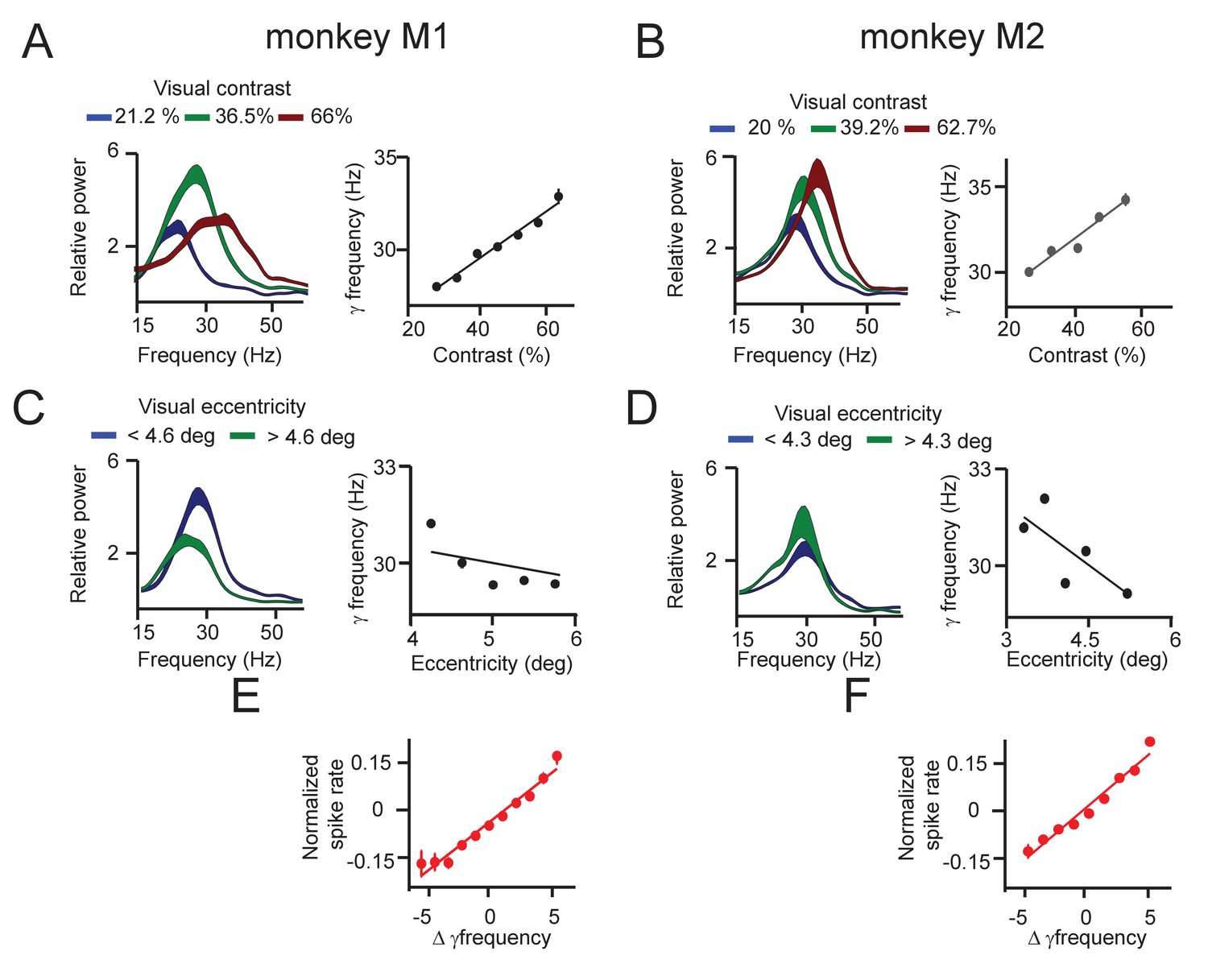
Effect of contrast and eccentricity on macaque V1 gamma frequency.
(A) On the left, the relative power spectra (15–55 Hz) of monkey M1 are shown for three representative grating contrasts (see Table S1) showing a monotonic increase in the preferred frequency range and a nonlinear power change with contrast. To the right, the dependence of (instantaneous) gamma frequency and local contrast is quantified. (B) The same as in A, but for monkey M2. (C) Left, the power spectra of contacts in monkey M1 with lower eccentricity (<4.6 deg) and higher eccentricity (>4.6 deg) are shown. A decrease in the peak frequency with higher eccentricity can be observed. This is quantified on the right in the plot of estimated gamma frequency and eccentricity. (D) The same as in C, but for monkey M2. (E) The MUA spike rate was similarly correlated with contrast and eccentricity as was gamma frequency in M1. In general, we observed that MUA spike rate difference among V1 locations predicted well changes in gamma frequency difference. (F) The same as in E, but for monkey M2.
Figure 2

Instantaneous frequency modulation.
(A) Example CSD (blue and red) traces recorded during visual stimulation from which gamma-band components were extracted using singular-spectrum decomposition. (B) We computed the phase difference (black) between signals 1 and 2 by computing the circular difference of their instantaneous phases. The instantaneous phase was derived by applying the Hilbert transform on the gamma-band components. (C) Taking the derivative, and scaling the result as the instantaneous frequency difference (ΔIF) gives the rate of phase precession. Notice the modulations over time. Note further that ΔIF variations are the result of IF variations occurring simultaneously at the two contact points that together constitute a contact pair. (D) Shows the ΔIF traces for all trials in a single session and stimulus condition for a single contact pair. (E) The ΔIF points (N = trial number*samples = 33*1800 = 59400) are plotted as a function of phase difference. A clear modulation of ΔIF values (blue line represents the mean) with phase difference can be observed showing that ΔIF modulations are not random. This means that phase precession depends on the momentary phase-difference (phase-relation) between contrasts. It is worth noting that the ΔIF values tend to be positive, which is related to the sign of the contrast difference and resulting detuning. If for the same pair the contrast difference had been reversed, ΔIF values would have tended to be negative.
Figure 3 with 2 supplements

Illustration of V1 gamma-band dynamics.
(A–C) Example 1 showing synchronization despite frequency difference (data from Monkey M1,~30 trials per condition). (A) Schematic figure of the contacts used from two laminar probes in V1. Below is a section of the stimulus grating with the corresponding RFs. The arrows’ thickness indicates the strength of contrast-dependent input to the corresponding V1 location. (B) Instantaneous frequency difference (ΔIF), equivalent to the phase precession rate, as a function of phase difference. Yellow dot indicates the modulation minimum, equivalent to the preferred phase difference, shading is ±SE (C) The phase difference probability distribution and phase-locking value (PLV). (D–F) Example 2; probes were closer and the gamma peak frequency difference was similar. Conventions as in A-C. (G–I) Example 3; same distance, reduced frequency difference. Compare B, E, H; the RF distance determined IF modulation amplitude, whereas contrast difference determined mean gamma frequency difference. Note that the instantaneous phase difference at which the instantaneous frequency difference is minimal (yellow dot) is smaller for greater amplitudes of instantaneous frequency difference variation (compare E, H to B).
Figure 3—figure supplement 1
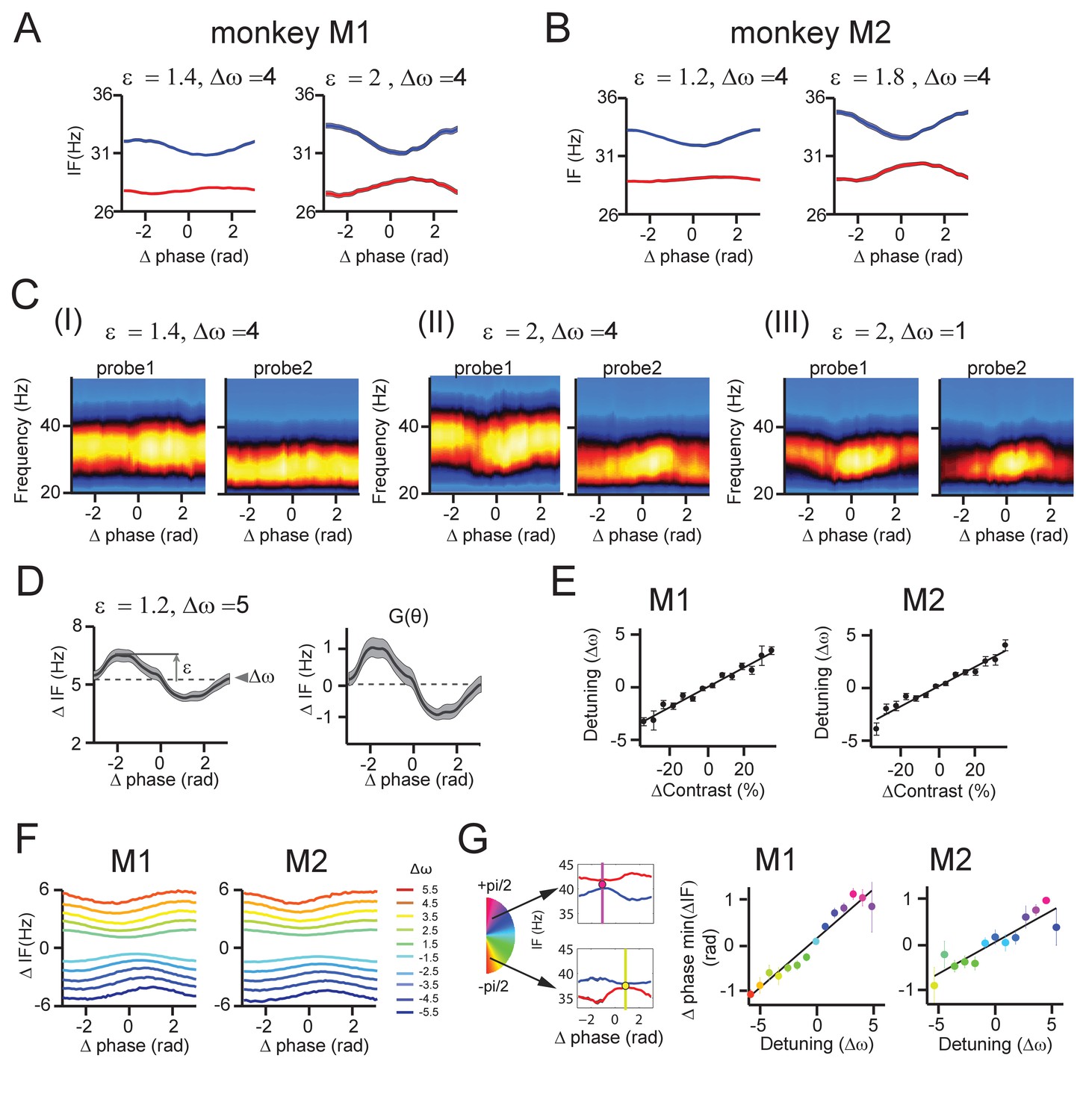
Instantaneous frequency modulations during gamma synchronization.
(A) Example plots of instantaneous frequency (IF) modulation by phase difference in monkey M1. The IF was estimated using the Hilbert transform. Left and right show two different modulation amplitudes. Blue and red represents the IF modulations of two respective contacts. Line thickness represents standard error. (B) The same as in A, but for monkey M2. (C) IF modulations are not method-dependent: Here, we computed the wavelet TFR and averaged the time points as a function of phase difference for a given contact pair (contact from probe 1 and probe2). This gives the phase difference averaged TFRs. In I-III we show different examples (from monkey M1). Clear modulations oogical rhythms and the bf the preferred gamma frequency can be seen as a change of phase difference between the contacts. (D) The procedure for the estimation of the interaction function G(θ) is illustrated. For the given contact pair, the difference of the IF modulations by phase difference was computed, resulting in the left plot. The mean (dashed line) was defined as the detuning ∆ω, and ε was estimated as the amplitude. To get an estimate of G(θ), the modulation was subtracted by ∆ω and normalized by ε, giving the right plot. (E) The estimated detuning as a function of contrast difference between contact pairs for M1 (left) and M2 (right). Contrast values were estimated based on the RF position on the stimulus grating. Note that (F) population-averaged IF difference modulations as a function of detuning for monkey M1 (left) and M2 (right). (G) In the intermittent synchronization regime the mean phase difference is determined by the phase difference in which the contacts have their minimal frequency difference (illustrated as filled dots in the small plots to the left). In line with theory, we indeed observed that the phase difference with minimal frequency difference shifted with detuning ∆ω similarly to the measured mean phase difference.
Figure 3—figure supplement 2
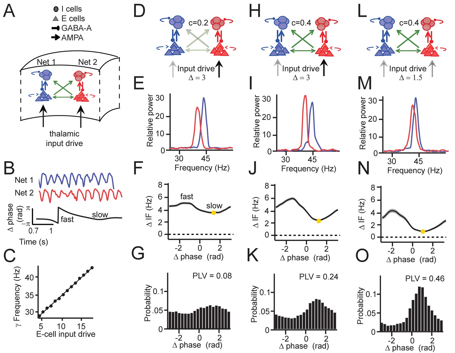
PING network simulations and intermittent synchronization.
(A) Two coupled pyramidal-interneuron gamma (PING) networks (Net 1 and Net 2). (B) Simulation output example network signals (red and blue) and phase difference θ (black) (C) The frequency of gamma in a single network depends on input strength. (D–G) Example 1 showing synchronization despite frequency difference. (D) Net 1 and Net 2 were relatively weakly coupled (c = 0.2, where c defines max synaptic connection strength of a uniform distribution [0, max]) and received a relatively large input difference. (E) Power spectra of the two networks showed different peak frequencies. (F) Instantaneous frequency difference (ΔIF), equivalent to phase precession rate, as a function of phase difference. Yellow dot indicates the modulation minimum equivalent to the preferred phase difference, shading is ±SE. (G) The phase difference probability distribution and phase-locking value (PLV). (H–K) Example 2; networks were more strongly connected (c = 0.4), gamma peak frequency difference was similar. Conventions as in D-G. (L–O) Example 3; same connection strength, yet reduced frequency difference. Compare F, J, N; the connection strength determined IF modulation amplitude, whereas input difference determined mean gamma frequency difference.
Figure 4

Theory of weakly coupled oscillators (TWCO).
(A) Schematic illustration of the model. Two limit-cycle oscillators (here symbolized by metronomes) that mutually interact with strength ε and dependent on function G(θ). Each oscillator has its own intrinsic frequency ω and the difference is termed detuning Δω. Each oscillator additionally had phase noise η. (B) The single differential equation used for analysis. (C) Output example from numerical simulation of Equation 1. The phase precession is shown above and the ΔIF is shown below. Notice the ΔIF modulations over time. (D) ΔIF modulations averaged as a function of Δphase. (E–J) Equivalent behavior as in the examples shown in Figure 3. Top panels E-G show the modulation of the instantaneous frequency difference as a function of phase difference. Note that the instantaneous Δphase at which the ΔIF is minimal (yellow dot) is smaller when the interaction strength is larger (compare F, G to E). Bottom panels (H–J) show the phase difference probability distributions. Black bars are numerical simulation results, red lines indicate the analytical solutions. (E.H) Large detuning and low interaction strength. (F,I) Large detuning and strong interaction strength. (G,J) Small detuning and strong interaction strength.
Figure 5 with 1 supplement
.General approach to derive and evaluate the theoretical predictions.
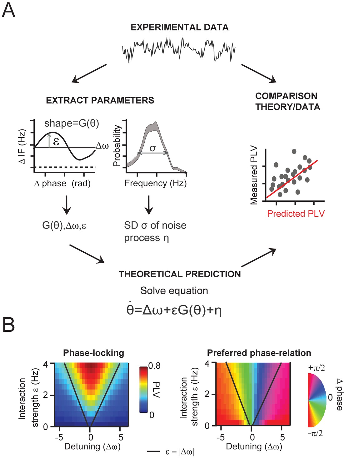
(A) Schematic illustration of the main procedure to derive and evaluate the theoretical predictions for gamma PLV. From the experimental data (instantaneous frequency difference, top) we needed to estimate the function G(θ) and the parameters ε, Δω and σ to solve Equation 1 (bottom), obtaining PLV predictions. We extracted (left) the function and parameters using observed (for G(θ),ε, Δω) and the gamma frequency distribution (for σ). We then solved Equation 1 for each contact pair and compared directly the predicted and observed PLV (right, where each point represents one condition and contact pair) (B) The prediction of the Arnold tongue. In the parameter-space of ε and Δω, a characteristic inverted triangular-shaped synchronization region is as expected from TWCO. Left is the analytically derived PLV from Equation 1 (where G(θ) being a sinusoid function and σ = 18 Hz). The black line represents the equality (ε=|∆ω|), which sharply defines the Arnold tongue in the noise-free case. Right the mean phase difference is mapped showing a gradual change of phase-difference along the detuning dimension.
Figure 5—figure supplement 1
Testing the accuracy of the interaction function reconstruction.
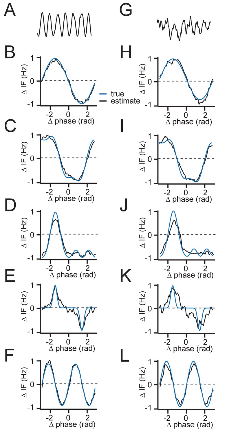
(A–F) Comparing the estimated G(θ) to the true G(θ) of two coupled phase-oscillators for different example shapes with high SNR (SNR = 12). (G–L) Same as (A–F), but for lower SNR comparable to V1 data (SNR = 3). (A/G) Example oscillatory trace (B/H) G(θ)=sin(θ) (C/I) G(θ) =-sin(θ)3-cos(θ) (D/J) G(θ) =-sin(θ)3-cos(θ)2 (E/K) G(θ) =-sin(θ)7 (F/L) G(θ)=sin(2θ).
Figure 6
Predicting V1 gamma synchronization in monkeys M1 and M2.
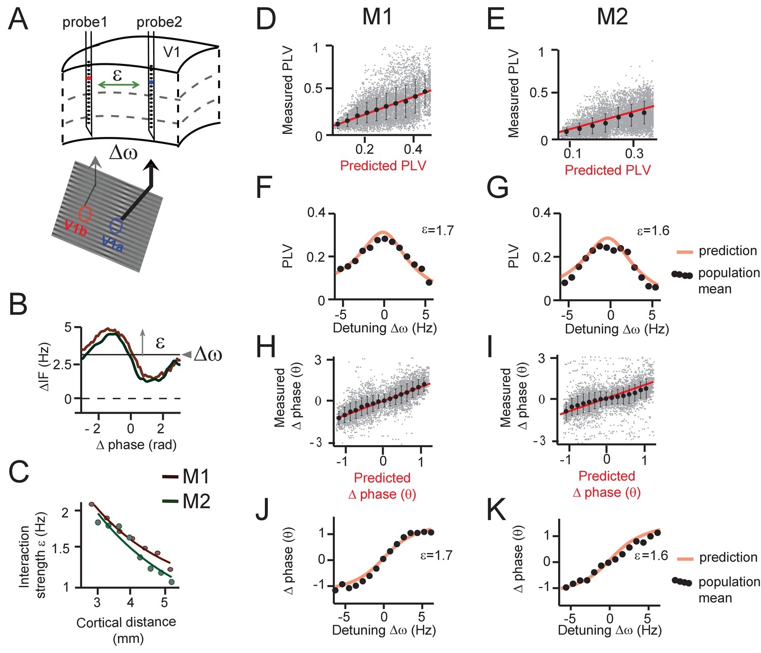
(A) Illustrative schema showing how detuning ∆ω and interaction strength ε of V1 gamma relate to local stimulus contrast and cortical distance respectively. (B) Example plots of averaged phase-dependent modulation of the instantaneous frequency difference (∆IF) used for estimating ε and ∆ω for monkey M1 (brown) and M2 (green). The shape of the modulation indicates the G(θ). (C) Plots showing that the interaction strength ε decreased with cortical distance in both monkeys M1 and M2. (D, E) Each gray dot represents one single contact pair data and condition plotted as function of the observed PLV (y-axis) and the analytical predictions (x-axis). The red line shows unity line. The black dots represent the population means binned according to predicted PLV (+-SE). (F, G) The observed PLV population means (dots) and the analytical predictions (gray line) as a function of detuning ∆ω for one level of interaction strength (ε = 1.7 in M1; ε = 1.6 in M2). (H, I) Same as in (D, E), but now for mean (preferred) phase differences. (J, K) Similar to (F, G), but now for mean phase difference.
Figure 7 with 4 supplements
Arnold tongues.
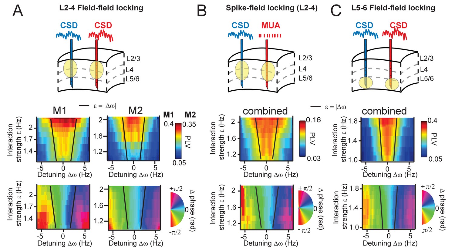
Combining different detuning ∆ω and interaction strengths ε, we observed a triangular region of high synchronization, the Arnold tongue. Black lines mark the predicted Arnold tongue borders as expected from the noise-free case (ε=|∆ω|). (A) CSD-CSD PLV from V1 layers 2–4 are shown for both monkeys. Notice the inverted triangular shape of PLV values. Below, the mean phase difference is mapped in the same parameter space exhibiting a clear gradient with detuning. (B) Same analysis as in (A), but using MUA spikes from one contact and the CSD from the other contact. Here combined for both monkeys. (C) The same analysis as in (A), but using contacts from deep layer 5–6 in V1. We separated the analysis for L5/6 and L2/3, because we found strong coherence within each group, but weak coherence between the groups (see more in the Appendix).
Figure 7—figure supplement 1

Applying the theory of weakly coupled oscillators to coupled PING networks.
(A) Two coupled pyramidal-interneuron gamma (PING) networks (Net 1 and Net 2). Detuning ∆ω was varied by excitatory input drive, whereas interaction strength ε was varied by inter-network connectivity strength. (B) An example plot of averaged phase-dependent modulation of the instantaneous frequency difference (∆IF) used for estimating ε and ∆ω. The shape of the modulation indicates the G(θ). (C) The simulation PLV at different detuning values ∆ω (dots colored by PLV) at a single interaction strength value (ε = 1.7) was well predicted by the model (gray line). (D) The PLV at many interaction strengths and detuning values mapped the Arnold tongue. Black lines mark the predicted Arnold tongue borders in the noise-free case (ε=|∆ω|). (E–F) As (C–D), but for preferred phase difference θ.
Figure 7—figure supplement 2
Arnold tongue mapping for CSD-MUA and MUA-MUA signals.
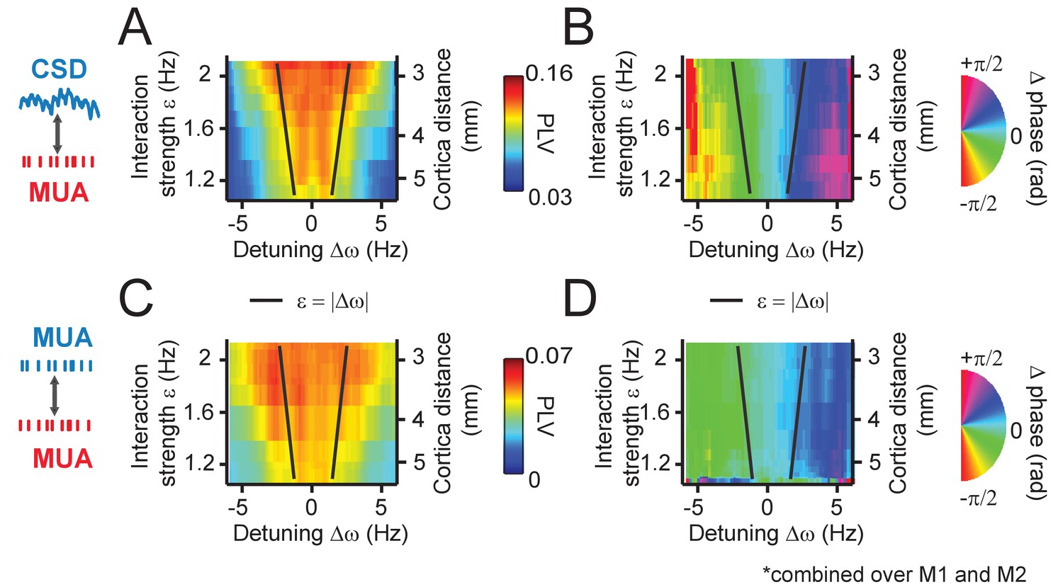
(A) For each contact pair, we selected the CSD signal from one contact and the MUA signal from the other contact for computing PLV as a function of detuning ∆ω and interaction strength ε/cortical distance. We observed a similar Arnold tongue in PLV as observed for CSD-CSD analysis. (B) The same as in A, but for mean phase difference. (C) The same analysis as in A, but for MUA-MUA signals. We also observed an Arnold tongue for MUA-MUA PLV. Notice that the MUA signals had much lower SNR than the CSD signals. (D) As in C, but for phase difference.
Figure 7—figure supplement 3
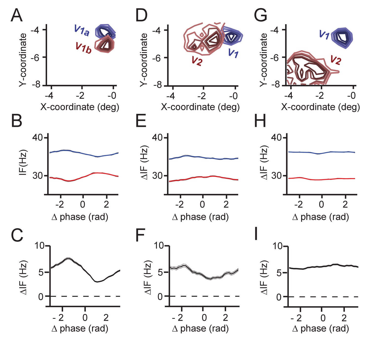
Phase-dependent instantaneous frequency modulation (and hence interaction strength ε) decreases with receptive field distance (and hence anatomical connectivity strength).
(A) The receptive fields of an example contact V1 pair (monkey M1). Contours represent the 50–90% percentiles of evoked responses during receptive field mapping. (B) The corresponding phase-difference dependent IF modulations for the V1 contact pair. (C) The resultant IF difference modulation. (D) Same as A, but now for a V1-V2 contact pair. V2 contact was from a deep contact of the laminar probe reaching V2 beneath of V1. (E) Same as (B), but now for V1-V2 pair. (F) Same as (C), but for the V1-V2 pair. (G) Same as (D), but now a V1-V2 pair with more distant receptive fields. (H–I) Same as (E–F).
Figure 7—figure supplement 4

Gamma amplitude modulation as a function of phase-difference.
(A) CSD gamma amplitude modulation from monkey M1 averaged over the two contacts for a given pair with modulation strength expressed in percent change from the mean (y-axis) and as a function of phase difference (x-axis). From left to right the interaction strength is increased (cortical distance decreased). We observed small- to medium-sized/intermediate modulation amplitudes of gamma amplitude. The modulation strength increased with interaction strength ε. Line thickness represents SE. (B) The same as in A, but for monkey M2. (C) Quantification of the gamma amplitude modulation in two coupled simulated PING networks. As for the monkey data, we observed systematic amplitude modulations that increased with interaction strength (synaptic connectivity). Line thickness represents the standard error of the instantaneous frequency for a given phase difference.
Figure 8

Same analysis as in Figure 7, but applying (non-stationary) granger causality directionality measure (X→ Y vs X ← X).
In line with phase-difference maps, the directionality influence flips as a function of detuning for monkey M1 (left) and M2 (right).
Figure 9
Summary of the main findings.
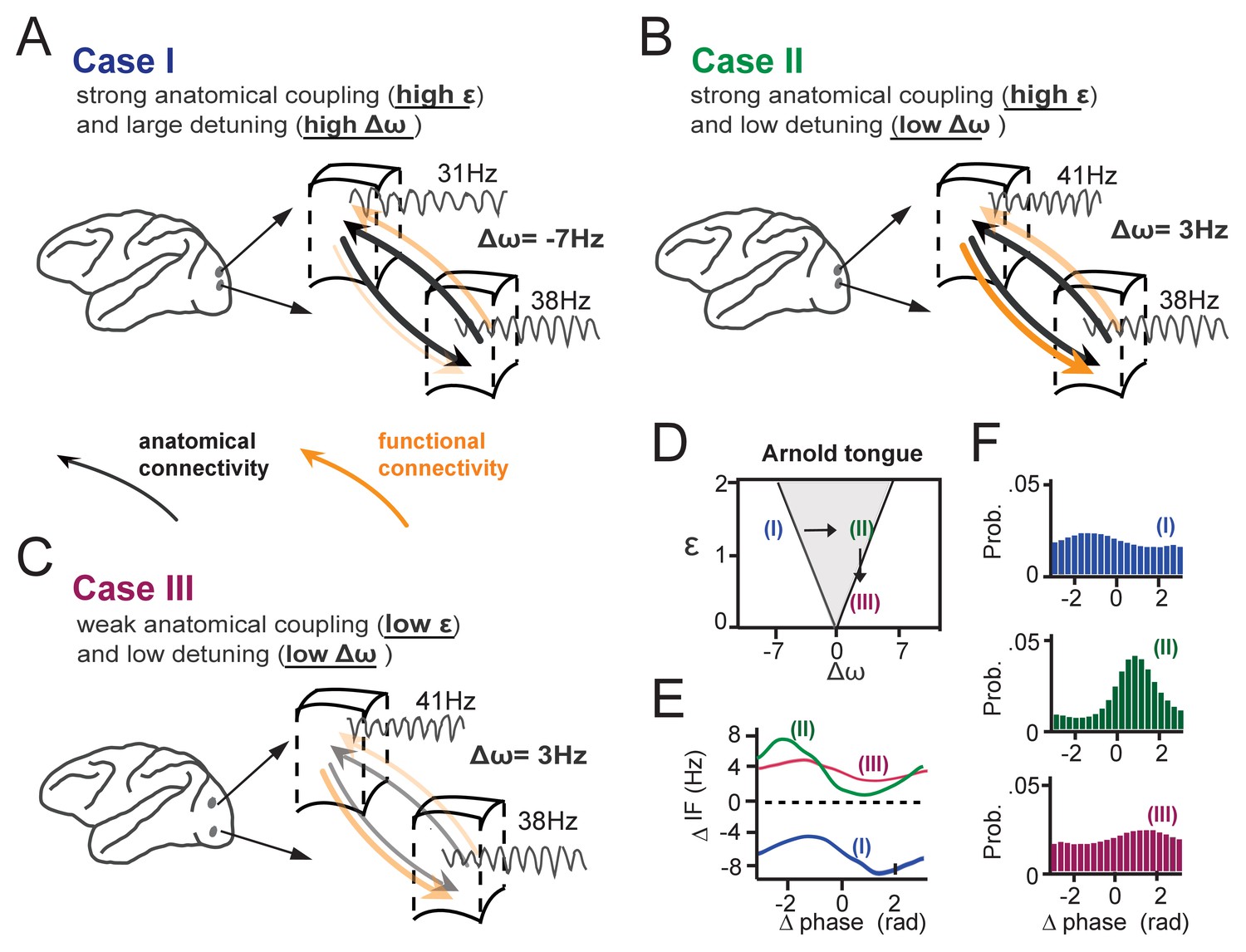
(A-C) Three cases of cortical gamma-band interactions are used for illustration (A) In case I, two cortical locations have strong anatomical connections (black thick arrows, high interaction strength ε) and a large detuning Δω. This results in low functional interaction (orange arrows). (B) In case II, anatomical connections are as high as in (A), but detuning is low. This leads to strong functional interactions. The location with higher frequency functionally dominates the location with lower frequency. (C) In case III, there is the same low detuning as in (B), but with low anatomical connectivity. This results again in low functional interaction. (D) The three cases represented in relation to the Arnold tongue. Only case II is within the Arnold tongue. Moving out of the Arnold tongue by a change in Δω (from II to I) or a change in ε (from II to III) strongly reduces synchronization. (E) The instantaneous frequency difference modulations (ΔIF(θ)) as a function of phase-difference for the three examples. (F) The corresponding phase-difference probability distributions.
Tables
Table 1
Range of contrast difference conditions used for the experimental task for monkeys M1 and M2.
The top sub-table shows the contrast difference conditions (in %) used for M1, and the bottom sub-table shows the values for M2.
| Contrast difference condition (monkey M1) | |||||||||
|---|---|---|---|---|---|---|---|---|---|
| Range | 44.7 | 35.9 | 24.8 | 13.3 | 0 | −13.3 | −24.8 | −35.9 | −44.7 |
| RF 1 | 66 | 58.6 | 51.7 | 44.3 | 36.5 | 31 | 27 | 22.7 | 21.2 |
| RF 2 | 21.2 | 22.7 | 27 | 31 | 36.5 | 44.3 | 51.7 | 58.6 | 66 |
| Contrast difference condition (monkey M2) | |||||||||
| Range | 42.7 | 34 | 24.5 | 13.6 | 0 | −13.6 | −24.5 | −34 | −42.7 |
| RF 1 | 62.7 | 57.5 | 52.2 | 46 | 39.2 | 32.5 | 27.7 | 23.5 | 20 |
| RF 2 | 20 | 23.5 | 27.7 | 32.5 | 39.2 | 46 | 52.2 | 57.5 | 62.7 |
Additional files
-
Transparent reporting form
- https://doi.org/10.7554/eLife.26642.021
Download links
A two-part list of links to download the article, or parts of the article, in various formats.
Downloads (link to download the article as PDF)
Open citations (links to open the citations from this article in various online reference manager services)
Cite this article (links to download the citations from this article in formats compatible with various reference manager tools)
A quantitative theory of gamma synchronization in macaque V1
eLife 6:e26642.
https://doi.org/10.7554/eLife.26642


