Beyond excitation/inhibition imbalance in multidimensional models of neural circuit changes in brain disorders
- University of Bristol, United Kingdom
- Howard Hughes Medical Institute, Salk Institute for Biological Studies, United States
- Albert Einstein College of Medicine, United States
- David Geffen School of Medicine at UCLA, United States
- University of California at San Diego, United States
Figures
Figure 1

Mismatch between the E/I imbalance model’s unidimesionality and the multiple changes in circuit activity in Fragile-X mouse models.
(A) Schematic of standard E/I imbalance model as a unidimensional axis. Fragile-X Syndrome and autism have been associated with an excess of excitation (Gibson et al., 2008; Lee et al., 2017; Nelson and Valakh, 2015), while Rett Syndrome has been associated with an excess of inhibition (Dani et al., 2005). (B) Diagram of a generic neural circuit, showing an excitatory and an inhibitory population of neurons and their interconnections. Although the E/I imbalance model implicitly groups all components as either excitatory (red) or inhibitory (blue), in principle any component could separately be altered in brain disorders, and may have a distinct effect on circuit function. (C) Upper left, example Ca2+ imaging dF/F raster plots from a single animal from each of two genotypes, WT and Fmr1 KO, and three age groups, P9–11, P14–16 and P30–40. In each case, 3 min of data are shown from 40 neurons. Right and lower left, mean firing probability, standard deviation of firing probabilities, and mean pairwise correlation across all neurons. Same data in scatter plots lower left and bar charts right. * indicates significant difference in group means at p<0.05, by bootstrapping.
Figure 2
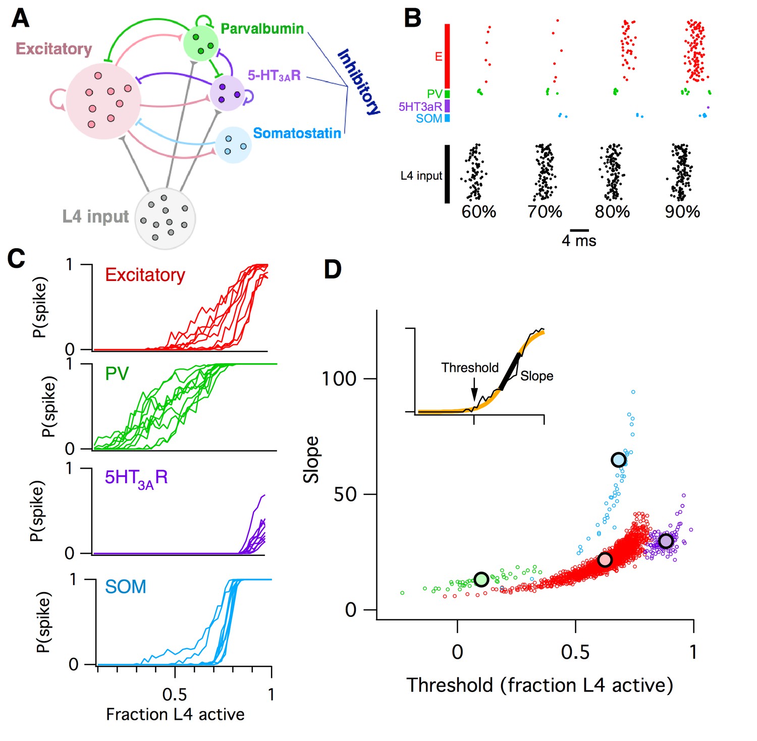
Computational model of L2/3 mouse somatosensory cortex.
(A) Schematic diagram of computational circuit model. (B) Example raster plots of spiking responses from a subset of neurons from each cell type (colors as in panel A), for varying fractions of L4 activated (black). (C) Probability of spiking as a function of the fraction of L4 neurons activated. Each curve represents the response probability of a single neuron, averaged over multiple trials and multiple permutations of active L4 cells. (D) Each circle plots the fitted logistic slope and threshold values for a single neuron in the simulation. Circle color indicates cell type: red is excitatory, green is PV inhibitory, purple is 5HT3AR inhibitory, blue is SOM inhibitory. Large black circles indicate mean for each cell-type. Inset shows an example fitted logistic response function (orange) to the noisy simulation results from a single excitatory neuron (black).
Figure 3
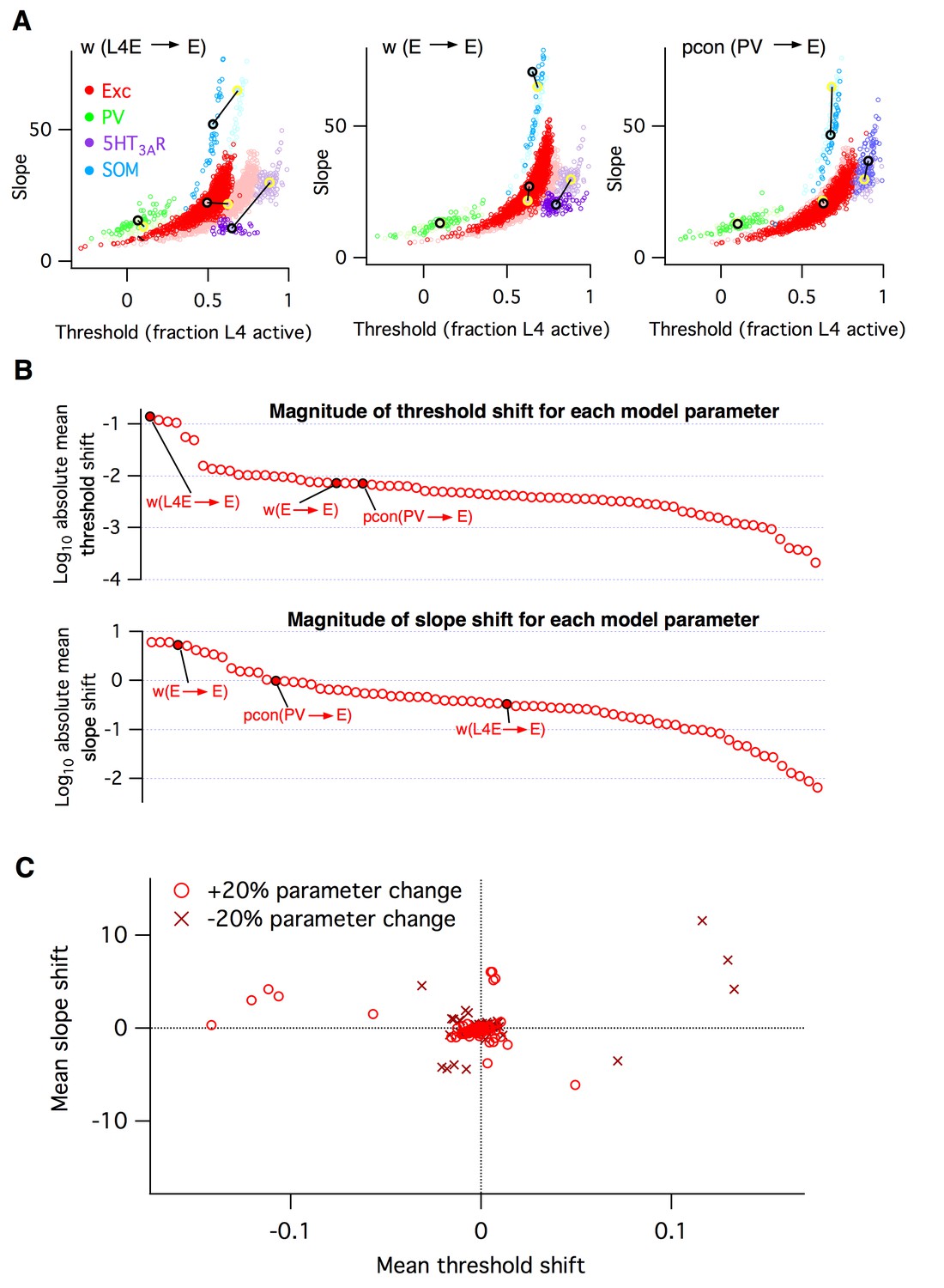
Heterogeneous effects of varying L2/3 parameters on the circuit input-output function.
(A) Shifts in the distribution of fitted slope and threshold parameters as a result of increasing the strength of synapses from L4 to L2/3 E neurons (left), increasing the strength of recurrent synapses between L2/3 E neurons (center), or increasing the connection probability between L2/3 PV interneurons and E neurons (right). Transparent circles represent values for default network, heavy circles for altered network. The default and altered group means are large yellow and black open circles, respectively. (B) Absolute values of mean shifts in threshold (upper plot) and slope (lower plot) for Excitatory neurons arising from increasing the value of each parameter by +20%. The three example parameters from panel A are labeled and indicated as filled red circles. Note that data are presented on a log10 scale. (C) The shift in mean slope-threshold parameter values for E neurons from the default network values, in response to each of the 76 circuit parameter alterations. Light red circles indicate +20% increase in parameter value; dark red crosses indicate a −20% decrease in parameter value.
Figure 4
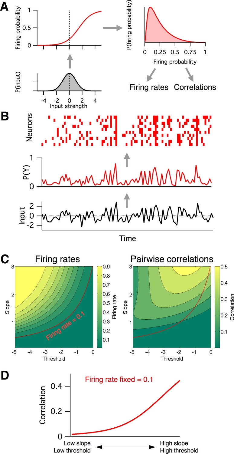
Firing rates and pairwise correlations from the logistic response model.
(A) Logistic model components. We assume a normally distributed input drive (gray distribution, bottom left), which is passed through the neuron’s probabilistic spike input-output function (red curve, top left), which results in a distribution of spike probabilities (top right) that are determined by the input-output function’s slope and threshold parameters. From the output distribution, we can directly calculate the mean firing rate and correlation between a pair of such neurons (Materials and methods). (B) Example spikes from the logistic model. The bottom trace (black) shows examples inputs over time drawn randomly from the same normal distribution. This is transformed to spike probability at each time point (red trace). Example spike trains can then be generated from the spike probability trace by drawing Bernoulli samples with the specified probabilities (red ticks, top). If each neuron’s spike train is conditionally independent given the same spike probabilities, we can see correlations in their spike trains. (C) Calculated mean firing rate (left) and pairwise correlation (right) color maps as a function of the logistic threshold (x-axis) and slope (y-axis) parameters. Contours indicate lines of fixed firing rate or correlation in the 2D slope-threshold space. (D) Pairwise correlation values along the slope-threshold contour for firing rate = 0.1.
Figure 5 with 2 supplements

Fragile-X fits from logistic model.
(A) Example samples from the fitted logistic models, corresponding to the six groups shown in panel A. Inset shows group mean fitted logistic function, dashed vertical line represents zero. (B) Fitted logistic mean slope and mean threshold values for data from each WT (black circles) and Fmr1 KO (red circles) animal. Values overlaid on same firing rate (top) and correlation (bottom) maps from Figure 4C. (C) Shift in mean logistic slope and threshold values from WT to KO for P9–11 (orange), P14–16 (red) and P30–40 (brown). Grey ellipses represent 95% confidence intervals (Materials and methods).
Figure 5–figure supplement 1

Agreement between population logistic model activity statistics and raw data statistics.
Black circles are WT, red are Fmr1 KO. Each data point corresponds to a recording from a single animal. Each plot shows model prediction versus raw data target value. Plots in each row correspond to data from a different age group (P9–11, P14–16, and P30–40), and each column corresponds to one of the three target activity statistics (mean firing rate, s.d. in firing rate, and mean pairwise correlation). Blue line is identity.
Figure 5–figure supplement 2
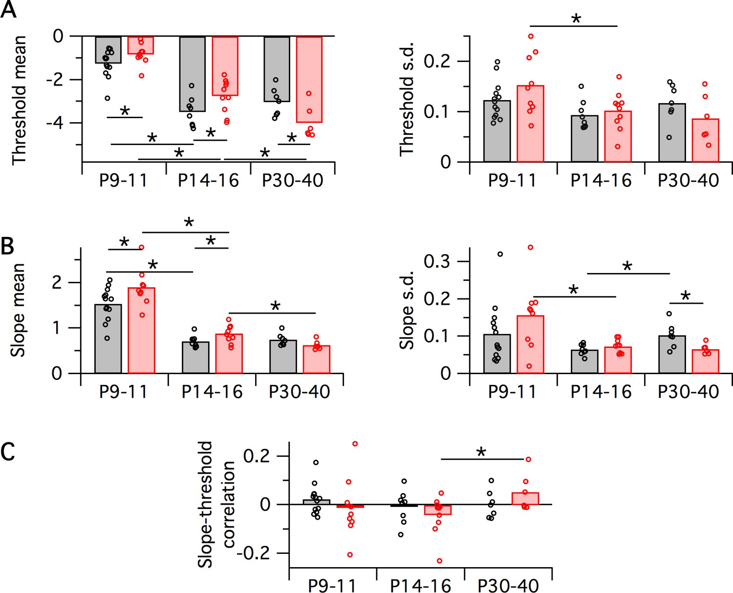
Variation in population logistic model parameter fits with developmental age group and genotype.
Black symbols are WT, red are Fmr1 KO. Each data point corresponds to a recording from a single animal, bars correspond to group means. In all cases, horizontal bar with asterisk indicates a significant difference in group means (p<0.05 via bootstrapping). (A) Logistic threshold parameter mean (left) and s.d. (right). (B) Logistic slope parameter mean (left) and s.d. (right). (C) Slope-threshold correlation parameter.
Figure 6
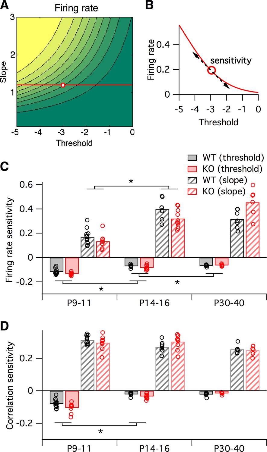
Sensitivity of firing rate and correlations with respect to logistic model parameters, local to the parameter fit for each animal.
(A–B) Sensitivity to a parameter is calculated about a given point in parameter space. In this hypothetical example, we plot a slope-threshold parameter fit at the red circle on the firing rate contour map (A). The firing rate varies non-linearly if the threshold is varied away from this point (B). Sensitivity is calculated as the local derivative, or slope of the tangent, about the target point. (C–D) Sensitivity of firing probability (C) and pairwise correlations (D) to change in threshold (solid bars) and slope (striped bars) parameters of logistic model, about the fitted parameter values for each animal (circles) displayed in Figure 5B. Bars represent group means. Each statistical test compares the mean values between adjacent pairs of age groups, where the data were pooled between genotypes.
Figure 7 with 1 supplement
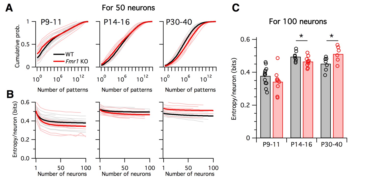
Differing trajectories of WT and KO entropy across development.
(A) Cumulative probability mass as a function of the number of patterns. Patterns ordered from most probable to least probable. Thin lines are mean across many randomly-chosen 50-neuron subsets from a given animal, and thick lines represent means across all animals of a given genotype. (B) Entropy per neuron as a function of the number of neurons analyzed. Thin lines are mean across many randomly chosen subsets for a given animal, thick lines are group mean of double exponential fits to the data (see Materials and methods). Age groups (left to right) are as in panel A. (C) Estimated entropy/neuron for 100 neuron populations. Circles represent individual animals, bars are group means.
Figure 7–figure supplement 1
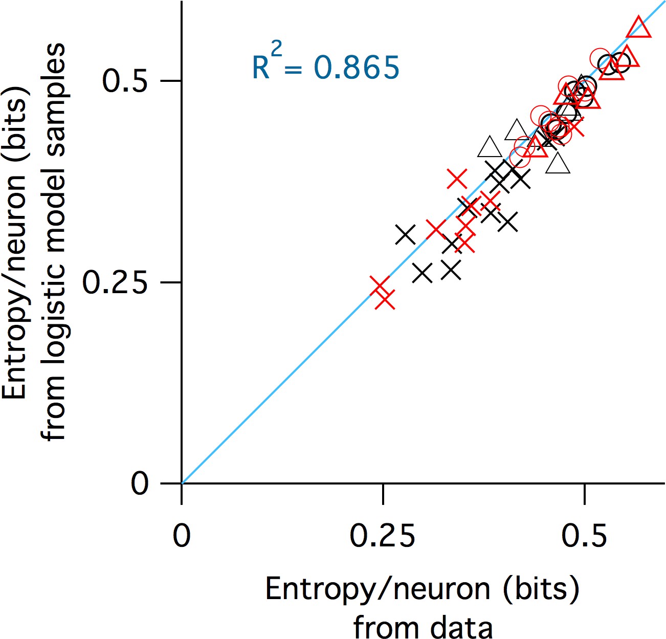
Agreement between entropy estimated from raw data with entropy estimated from samples from fitted logistic models.
Black symbols are WT, red are Fmr1 KO. Crosses are P9–11, circles P14–16, triangles P30–40. Blue line is identity. The R2 value of the identity line is reported in the inset, which represents the fraction of the variance of the logistic model entropies explained by this line.
Tables
Key resources table
| Reagent type (species) or resource | Designation | Source or reference | Identifiers |
|---|---|---|---|
| strain, strain background (mus musculus) | c57bl/6J strain of wild type mice | Jackson Labs | IMSR_JAX:000664 |
| genetic reagent (mus musculus) | Fmr1 knockout mouse on a c57 background | William Greenough (originally from Dutch-Belgian Fragile X Consortium) | RRID:MGI:2665400 |
| chemical compound, drug | OGB1 AM (Oregon Green BAPTA-1 AM) | Molecular Probes (ThermoFisher Scientific) | |
| Software, algorithm | ImageJ | NIH | RRID:SCR_003070 |
| software, algorithm | BRIAN Simulator | http://briansimulator.org | RRID:SCR_002998 |
| software, algorithm | MATLAB | http://www.mathworks.com/products/matlab | RRID:SCR_001622 |
Table 1
L2/3 computational circuit model parameters and mean slope and threshold shifts.
https://doi.org/10.7554/eLife.26724.013| Parameter | Value | Source | +20% effect on slope, thresh | Parameter | Value | Source | +20% effect on slope, thresh |
|---|---|---|---|---|---|---|---|
| NE | 1700 | [1] | slope: 6.4 × 10⁻³ thresh: 5.16 | pconI5htE | 0.465 | [2] | slope: −3.25 × 10⁻³ thresh: −0.103 |
| NIpv | 70 | [1] | slope: 4.3 × 10⁻³ thresh: −1.51 | pconI5htIpv | 0.38 | [2] | slope: −7.13 × 10⁻³ thresh: −0.298 |
| NI5ht | 115 | [1] | slope: −0.0104 thresh: −0.58 | pconI5htI5ht | 0.38 | [2] | slope: 6.07 × 10⁻⁴ thresh: 0.175 |
| NIsom | 45 | [1] | slope: −0.001 thresh: −0.83 | pconI5htIsom | 0 | No data | Not tested |
| NEL4 | 1500 | [1] | slope: −0.106 thresh: 3.43 | pconIsomE | 0.5 | [5] | slope: −6.29 × 10⁻³ thresh: −0.8919 |
| VrestE | −68 mV | [2] | slope: 0.049 thresh: −6.09 | pconIsomIpv | 0 | No data | Not tested |
| VrestIpv | −68 mV | [2] | slope: −0.016 thresh: −0.963 | pconIsomI5ht | 0 | No data | Not tested |
| VrestI5ht | −62 mV | [2] | slope: −9.48 × 10⁻⁴ thresh: 0.205 | pconIsomIsom | 0 | No data | Not tested |
| VrestIsom | −57 mV | [3] | slope: 3.58 × 10⁻³ thresh: 0.034 | prelEL4E | 0.25 | No data | slope: −0.112 thresh: 4.21 |
| VthE | −38 mV | [2] | slope: −3.76 × 10⁻³ thresh: −0.381 | prelEL4Ipv | 0.25 | No data | slope: 0.0103 thresh: 0.682 |
| VthIpv | −37.4 mV | [2] | slope: 3.87 × 10⁻³ thresh: 0.221 | prelEL4Isom | 0.25 | No data | slope: −2.06 × 10⁻³ thresh: −0.537 |
| VthI5ht | −36 mV | [2] | slope: −1.12 × 10⁻³ thresh: 0.013 | prelEE | 0.25 | No data | slope: 4.99 × 10⁻³ thresh: 6.074 |
| VthIsom | −40 mV | [3] | slope: −3.26 × 10⁻³ thresh: −0.083 | prelEIpv | 0.25 | No data | slope: −4.04 × 10⁻⁴ thresh: 0.163 |
| RinE | 160 MΩ | [2] | slope: 1.95 × 10⁻³ thresh: −0.283 | prelEI5ht | 0.25 | No data | slope: −9.32 × 10⁻³ thresh: −0.532 |
| RinIpv | 100 MΩ | [2] | slope: −8.38 × 10⁻³ thresh: −0.283 | prelEIsom | 0.25 | No data | slope: −7.32 × 10⁻³ thresh: −0.3847 |
| RinI5ht | 200 MΩ | [2] | slope: −3.87 × 10⁻³ thresh: −0.653 | prelIpvE | 0.25 | No data | slope: 1.03 × 10⁻² thresh: −0.941 |
| RinIsom | 250 MΩ | [4] | slope: 7.55 × 10⁻³ thresh: 0.465 | prelIpvIpv | 0.25 | No data | slope: 1.21 × 10⁻³ thresh: −0.061 |
| τmE | 28 ms | [2] | slope: −9.59 × 10⁻³ thresh: 0.268 | prelIpvI5ht | 0.25 | No data | slope: −4.73 × 10⁻³ thresh: 0.011 |
| τmIpv | 21 ms | [2] | slope: 4.82 × 10⁻³ thresh: 0.027 | prelI5htE | 0.25 | No data | slope: −1.63 × 10⁻³ thresh: −0.379 |
| τmI5ht | 10 ms | [2] | slope: −5.09 × 10⁻³ thresh: −0.302 | prelI5htIpv | 0.25 | No data | slope: −3.41 × 10⁻³ thresh: −0.262 |
| τmIsom | 30 ms | [4] | slope: −2.89 × 10⁻³ thresh: −0.159 | prelI5htI5ht | 0.25 | No data | slope: 3.05 × 10⁻³ thresh: 0.123 |
| trefE | 55.5 ms | [2] | Not tested | prel,IsomE | 0.25 | No data | slope: −2.13 × 10⁻⁴ thresh: −0.65 |
| trefIpv | 5.4 ms | [2] | Not tested | wEL4E,mean | 0.8 mV | [1] | slope: −0.142 thresh: 0.342 |
| trefI5ht | 21.3 ms | [2] | Not tested | wEL4E,median | 0.48 mV | [1] | slope: −0.142 thresh: 0.342 |
| trefIsom | 20 ms | [3] | Not tested | wEL4Ipv,mean | 0.8 mV | =wELEL4E | slope: 3.61 × 10⁻³ thresh: 6.54 × 10⁻³ |
| τsynE,e | 2 ms | Typical | slope: 1.37 × 10⁻² thresh: −1.79 | wEL4Ipv,median | 0.48 mV | =wELEL4E | slope: 3.61 × 10⁻³ thresh: 6.54 × 10⁻³ |
| τsynE,i | 40 ms | [2] | slope: −7.29 × 10⁻³ thresh: 0.48 | wEL4Isom,mean | 0.8 mV | =wELEL4E | slope: 5.05 × 10⁻³ thresh: −0.329 |
| τsynIpv,e | 2 ms | Typical | slope: −9.79 × 10⁻³ thresh: −0.477 | wEL4Isom,median | 0.48 mV | =wELEL4E | slope: 5.05 × 10⁻³ thresh: −0.329 |
| τsynIpv,i | 16 ms | [2] | slope: 1.56 × 10⁻³ thresh: −0.097 | wEE,mean | 0.37 mV | [2] | slope: 7.44 × 10⁻³ thresh: 5.34 |
| τsynI5ht,e | 2 ms | Typical | slope: 4.52 × 10⁻³ thresh: −0.047 | wEE,median | 0.2 mV | [2] | slope: 7.44 × 10⁻³ thresh: 5.34 |
| τsynI5ht,i | 40 ms | [2] | slope: −3.82 × 10⁻³ thresh: −0.387 | wEIpv,mean | 0.82 mV | [2] | slope: −3.77 × 10⁻⁴ thresh: −0.297 |
| τsynIsom,e | 2 ms | Typical | slope: −0.0126 thresh: −8.82 × 10⁻³ | wEIpv,median | 0.68 mV | [2] | slope: −3.77 × 10⁻⁴ thresh: −0.297 |
| τsynIsom,i | 40 ms | [2] | slope: −4.88 × 10⁻³ thresh: −0.301 | wEI5ht,mean | 0.39 mV | [2] | slope: −6.81 × 10⁻³ thresh: −0.46 |
| Ereve | 0 mV | Typical | slope: −0.056 thresh: 1.53 | wEI5ht,median | 0.19 mV | [2] | slope: −6.81 × 10⁻³ thresh: −0.46 |
| ErevEi | −68 mV | =VrestE | slope: 3.2 × 10⁻³ thresh: −3.77 | wEIsom,mean | 0.5 mV | No data | slope: −3.61 × 10⁻³ thresh: −0.359 |
| ErevIpvi | −68 mV | =VrestIpv | slope: −0.010 thresh: −0.617 | wEIsom,median | 0.4 mV | No data | slope: −3.61 × 10⁻³ thresh: −0.359 |
| ErevI5hti | −62 mV | =VrestII5ht | slope: 3.8 × 10⁻³ thresh: 0.132 | wIpvE,mean | 0.52 mV | [2] | slope: 6.41 × 10⁻³ thresh: −1.47 |
| ErevIsomi | −57 mV | =VrestIsom | slope: −4.2 × 10⁻³ thresh: −0.088 | wIpvE,median | −0.29 mV | [2] | slope: 6.41 × 10⁻³ thresh: −1.47 |
| pconEL4E | 0.15 | No data | slope: −0.121 thresh: 2.99 | wIpvIpv,mean | −0.56 mV | [2] | slope: −2.52 × 10⁻³ thresh: −0.345 |
| pconEL4Ipv | 0.15 | No data | slope: 1.38 × 10⁻³ thresh: 0.029 | wIpvIpv,median | −0.44 mV | [2] | slope: −2.52 × 10⁻³ thresh: −0.345 |
| pconEL4I5ht | 0 | No data | Not tested | wIpvI5ht,mean | −0.83 mV | [2] | slope: −4.24 × 10⁻³ thresh: −0.266 |
| pconEL4Isom | 0.15 | No data | slope: 7.62 × 10⁻³ thresh: −0.245 | wIpvI5ht,median | −0.6 mV | [2] | slope: −4.24 × 10⁻³ thresh: −0.266 |
| pconEE | 0.17 | [2] | slope: 5.86 × 10⁻³ thresh: 6.084 | wI5htE,mean | −0.49 mV | [2] | slope: −3.61 × 10⁻⁴ thresh: −0.018 |
| pconEIpv | 0.575 | [2] | slope: −1.17 × 10⁻³ thresh: −0.099 | wI5htE,median | −0.3 mV | [2] | slope: −3.61 × 10⁻⁴ thresh: −0.018 |
| pconEI5ht | 0.24 | [2] | slope: −6.44 × 10⁻³ thresh: −0.541 | wI5htIpv,mean | −0.49 mV | [2] | slope: −1.77 × 10⁻³ thresh: −0.187 |
| pconEIsom | 0.5 | [5] | slope: −4.37 × 10⁻³ thresh: −0.27 | wI5htIpv,median | −0.15 mV | [2] | slope: −1.77 × 10⁻³ thresh: −0.187 |
| pconIpvE | 0.6 | [2] | slope: 7.16 × 10⁻³ thresh: −1.049 | wI5htI5ht,mean | −0.37 mV | [2] | slope: −4.12 × 10⁻³ thresh: −0.416 |
| pconIpvIpv | 0.55 | [2] | slope: −2.61 × 10⁻³ thresh: −0.0456 | wI5htI5ht,median | −0.23 mV | [2] | slope: −4.12 × 10⁻³ thresh: −0.416 |
| pconIpvI5ht | 0.24 | [2] | slope: −2.81 × 10⁻³ thresh: −0.458 | wIsomE,mean | −0.5 mV | No data | slope: −0.013 thresh: −0.984 |
| pconIpvIsom | 0 | No data | Not tested | wIsomE,median | −0.4 mV | No data | slope: −0.013 thresh: −0.984 |
Additional files
-
Transparent reporting form
- https://doi.org/10.7554/eLife.26724.014
Download links
A two-part list of links to download the article, or parts of the article, in various formats.
Downloads (link to download the article as PDF)
Open citations (links to open the citations from this article in various online reference manager services)
Cite this article (links to download the citations from this article in formats compatible with various reference manager tools)
Beyond excitation/inhibition imbalance in multidimensional models of neural circuit changes in brain disorders
eLife 6:e26724.
https://doi.org/10.7554/eLife.26724


