Live tracking of moving samples in confocal microscopy for vertically grown roots
- Institute of Science and Technology Austria, Austria
Figures
Figure 1
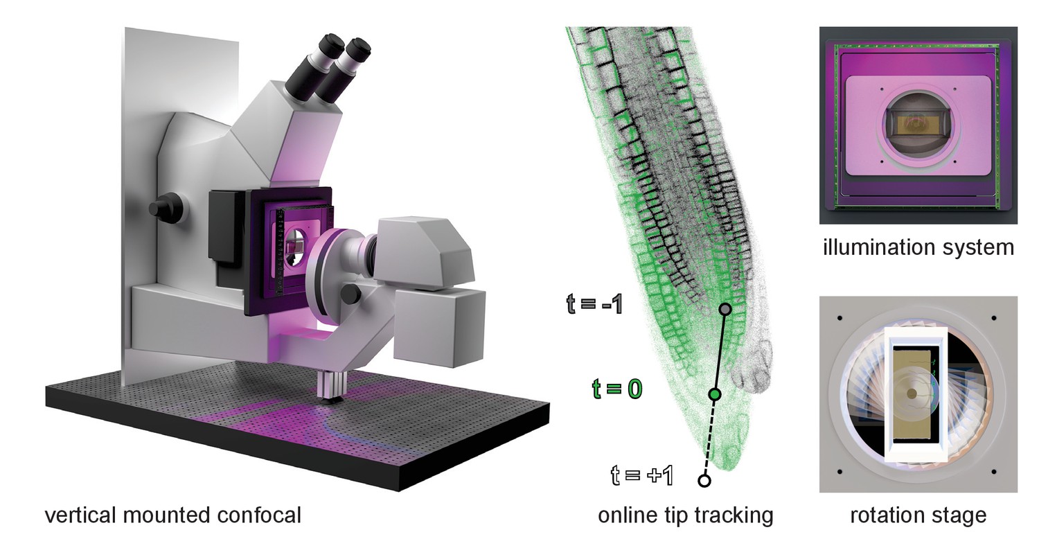
Overview of the vertical microscope setup.
The vertically mounted confocal microscope enables long-term imaging of plant roots growing along the gravity vector under controlled illumination. Growing root tips are tracked using the TipTracker MATLAB program. By turning the sample around the optical axis using the rotation stage, gravistimulation is applied to the growing root tips.
Figure 2
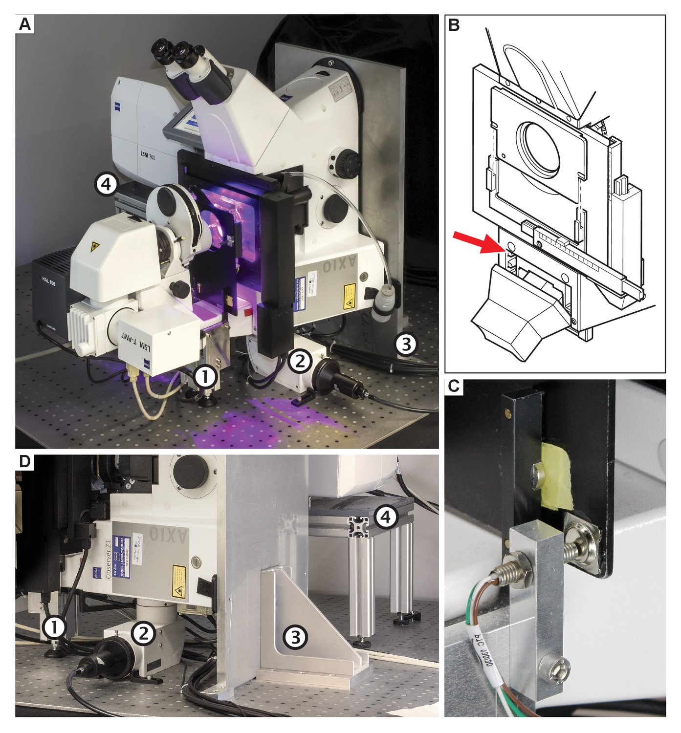
The vertically-mounted microscope setup.
The microscope body (Zeiss Axio Observer) was rotated by 90° and mounted to an optical table using a strong angle bracket. The scan head (Zeiss LSM 700) has been raised but retained its original orientation. (A) Photograph of the setup in our laboratory. (B) The laser safety mechanism. Since the transmitted light arm can no longer be reclined/tilted, the laser safety shield would limit the access to the sample. The reed switch (red arrow) was removed, and the screws holding the safety shield were replaced by pins and magnets. The reed switch was relocated to the bracket that holds the shield, depicted in (C). (D) Photograph showing the stand (1), the 90° adapter for wide field fluorescence excitation (2), the aluminium plate and mounting bracket (3), and the scan-head table (4).
Figure 3
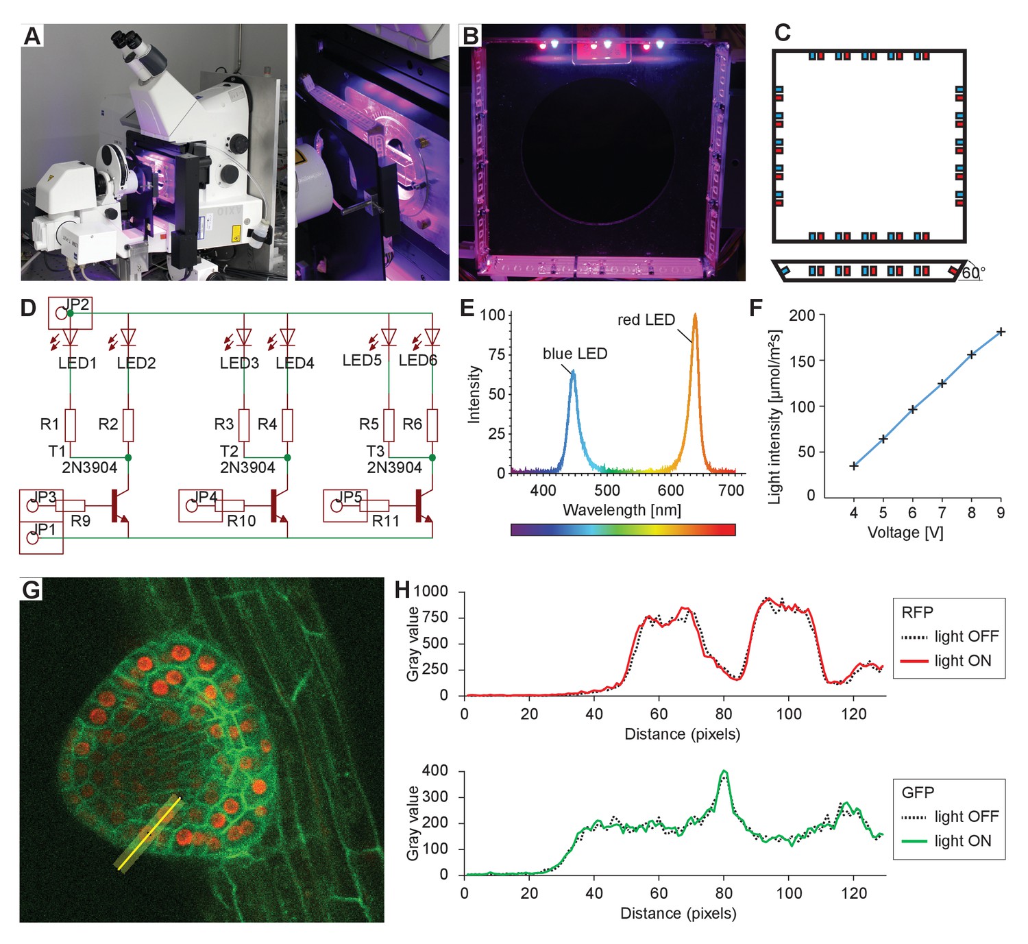
Integrated sample illumination setup.
(A) Photograph of the LED illumination system attached to the microscope. Red and a blue LED are arranged in a square. Each side of the square can be switched on/off individually for directional lighting. (B) Photograph from the sample side. (C) Schematic of the LED square arrangement. Each side is tilted by 60° toward the sample. We provide the board design file in the Supplementary file 1. (D) Schematic of the circuit diagram of one side of the lamp. LED: light-emitting diode, R: resistor, T: transistor, JP: pinhead. (E) The emission spectrum of the lamp. (F) The voltage can be adjusted in the range of 3.5–9.5 V. Resistors used to reach light intensities ranging from 40 to 180 μmol/m²/s: R1-8: 220 Ohm, R9-12: 1220 Ohm. (G) Single optical section recording of a lateral root primordium expressing GFP-plasma membrane marker UBQ10::YFP-PIP1;4 and RFP-nuclear UBQ10::H2B-RFP marker. Green fluorescence was collected between 490 and 576 nm, red fluorescence was collected between 560 and 700 nm. The fluorescence intensity profile of the yellow line (21 px width) is plotted in (H). (H) Intensity profile along the yellow line shown in (G) of the red and green channels with illumination system switched on or off, respectively, demonstrating that RFP/GFP imaging is not affected by the illumination.
Figure 4

Gravistimulation of samples using the sample rotation stage.
(A) Roots grow in chambered coverslips between the coverglass and a block of agar. (B) The sample chamber is placed in the rotation stage. The enlargement highlights the small screw mounting the sample chamber in the rotation stage, while the bigger screw fixes the rotation inset. (C) The chamber can be rotated around the optical axis inside the microscope inset which leads to a reorientation of the root with respect to the gravity vector. (D) The new positions of the root tips after rotations are calculated using a script to minimize the delay between rotations and imaging (Supplementary file 2). (E) and F) The construction of the sample rotation stage. The rotation stage is pressed in an inner Teflon ring (green ring), which is held together by an inner- and outer Teflon ring (red and blue) compressed by the front- and back aluminium plates. This arrangement provides smooth rotation of the sample. 3D files are provided in Supplementary file 1.
Figure 5
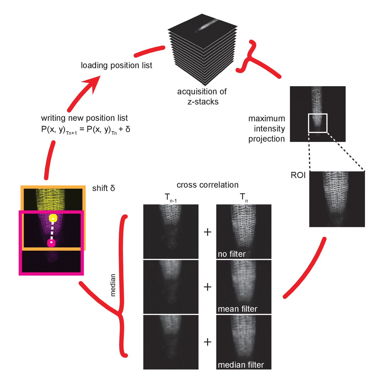
Working cycle of the TipTracker program.
A region of interest is selected from a maximum intensity projection of a z-stack. Mean and median filters are applied. A direct cross-correlation is performed between the current and the prior time point on the differently filtered and non-filtered images. Note that this procedure is purely based on the similarity of the images within the region of interest and makes no assumption about the sample. The median of the three results is used as the shift to make the calculation more robust. The calculated shift is added to the current position and is used as a prediction of the position of the root in the subsequent time point. The new position list is saved and then loaded at the start of the next acquisition time step.
Figure 6
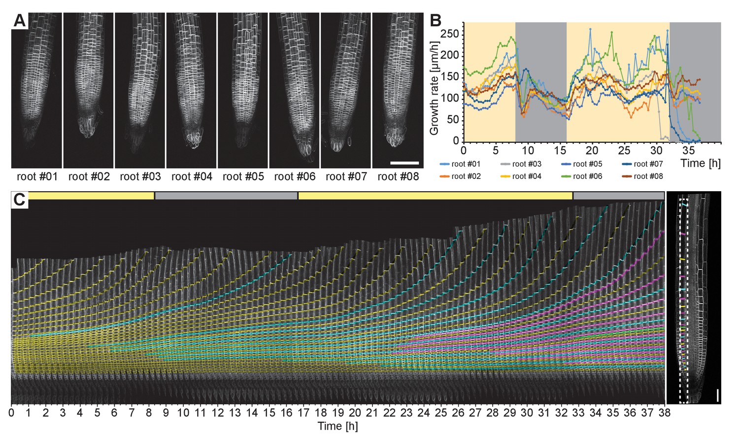
Time-lapse recording of eight Arabidopsis root tips expressing UBQ10::YFP- PIP1;4 over the course of 38 h.
(A) Maximum intensity projections of a single time point for the eight roots tracked. (B) Growth rates of the root tips were calculated from the output of the TipTracker program. The yellow and grey areas indicate when the LED illumination was on or off, respectively. (C) Cell division and elongation are visualized for the root #5. Each new cell wall is highlighted so that the original cell walls are in yellow, the second generation of the walls is in cyan, the third generation is in magenta, and the fourth generation in green. The last image of the series is shown on the right side. A stack of 14 images (x/y/z: 1400 × 1400 × 14 pixels, voxelsize: 0.457 × 0.457 × 2.5 μm³) was captured every 20 min for a period of 38 h 20 min using the Plan-Apochromat 20x/0.8 air objective lens. Scale bars: (A) 100 μm, (C) 40 μm.
Figure 7
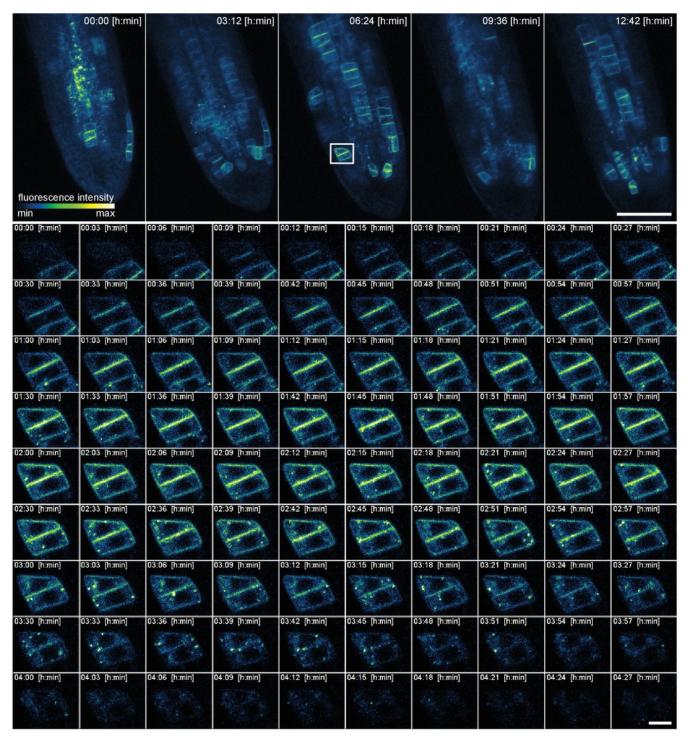
High spatio-temporal resolution time lapse recording of a 5-day-old Arabidopsis root tip expressing KNOLLE::GFP:KNOLLE.
The upper panel shows the maximum intensity projection of five time points out of 255. The appearance and disappearance of the fluorescent fusion protein during cytokinesis of a single cell is depicted in the lower panel. A stack of 10 images (x/y/z: 1448 × 1448 × 10 pixels, voxelsize: 0.138 × 0.138 × 2 μm³) was captured every 3 min for a period of 12 h and 42 min using the Plan-Apochromat 40x/0.95 air objective lens. Scale bars: 100 μm upper panel, 10 μm lower panel.
Figure 8
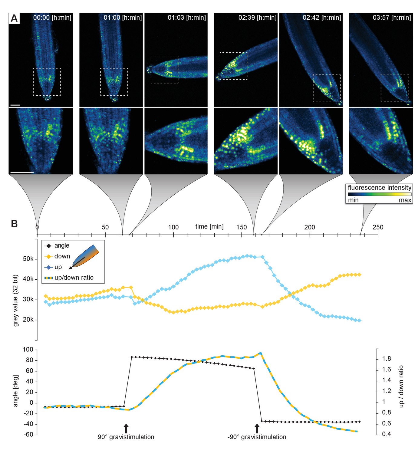
Recording of the gravitropic response of a 5-day-old Arabidopsis root tip expressing the DII-VENUS marker.
Initially, the root growth was followed for 1 h in the vertical position. Subsequently, the plants were gravistimulated by a 90° rotation (clockwise) and imaged for 1 h 36 min. Finally, the plants were rotated back (90° counter clockwise) and imaged for another 1 h 15 min. Three roots were imaged simultaneously, see also the Video 5. (A) Sum intensity projections of six time points out of 80. (B) Upper diagram shows the fluorescent intensity on the upper/left side (blue line) compared the lower/right side of the root tip (yellow line). The lower graph shows the root tip angle and the ratio of fluorescence intensity upper / lower side. A stack of five images (x/y/z: 1024 × 1024 × 5 pixels, voxelsize: 0.625 × 0.625 × 3 μm³) was captured every 3 min for a period of 4 h using the Plan-Apochromat 20x/0.8 air objective lens. Scale bars: 50 μm.
Figure 9
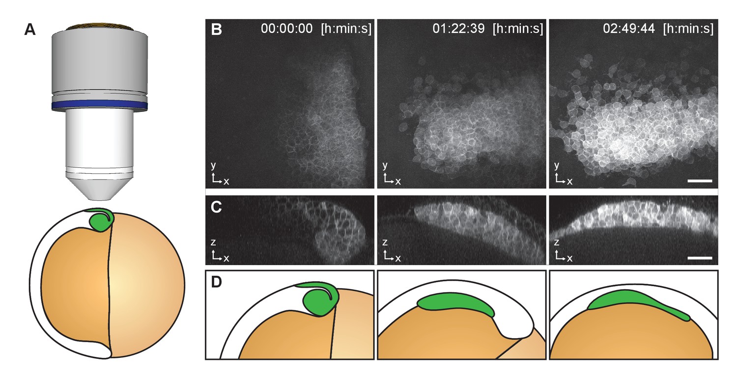
Imaging of Zebrafish prechordal plate using TipTracker with the LavisionBiotech TriM Scope II.
(A) Schematic representation of the shield stage of a six hpf gsc::mEGFP Zebrafish embryo. Membrane bound EGFP is expressed in the prechordal plate (ppl) cells that form the shield (green). (B) Maximum intensity projections of three time points out of 78 show the gsc::mEGFP expression over time. (C) A transversal section (3.40 μm width maximum intensity projection) shows ppl cells ingression and subsequent migration. See also Video 8. (D) Schematic representation of gsc::mEGFP expressing cells ingression and migration between shield stage and 90% epiboly stage (9 h post fertilization). A stack of 50 images (x/y/z: 1024 × 1024 × 50 pixels, voxelsize: 0.342 × 0.342 × 3.0 μm³) was captured every 2 min 15 s for a period of 2 h 50 min using the Zeiss Plan-Apochromat 20x/1.0 air objective lens. Time 0 corresponds to six hpf. Scale bars: (B, C) 50 μm.
Figure 10
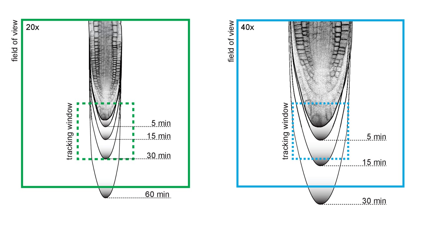
Root tip growth rate and tracking window.
For successful tracking, it is recommended to use a spatio-temporal resolution in relation to the expected growth rate of the root. The maximum growth rate of Arabidopsis primary root tip can be 300 μm/h. Black gradient lines indicate how much a root tip might grow after certain periods of time. The dashed square indicates the tracking area which is 1/3 of field-of-view’s dimensions (20x = 213 μm², 40x = 106 μm²).
Videos
Video 1
3D model of the vertical mounted confocal microscope.
https://doi.org/10.7554/eLife.26792.004
Video 2
Time series of eight Arabidopsis root tips recorded over 38 h.
https://doi.org/10.7554/eLife.26792.009
Video 3
Single slice of root tip number 5 of Video 2.
https://doi.org/10.7554/eLife.26792.010
Video 4
High-resolution time series of a root tip expressing KNOLLE::GFP-KNOLLE.
https://doi.org/10.7554/eLife.26792.012
Video 5
24 h recording of six Arabidopsis root tips expressing KNOLLE::GFP-KNOLLE.
https://doi.org/10.7554/eLife.26792.013
Video 6
Gravistimulation experiment.
Time series of three Arabidopsis root tips expressing the auxin response marker DII-Venus.
Video 7
Time series of Zebrafish prechordal plate using TipTracker with the LavisionBiotech TriM Scope.
https://doi.org/10.7554/eLife.26792.017
Video 8
Time series of a root tip growing along another root demonstrating the robustness of tracking in a spectacular way.
https://doi.org/10.7554/eLife.26792.019
Video 9
Time series of a root tip growing away from the objective lens inside the gel.
As a result, the root tip is no more in focus but the blurred root is still tracked by TipTracker.
Additional files
-
Supplementary file 1
Hardware.
(1) Board design of the illumination system. (2) Mounting plate for Axio Observer. (3) Modification of the laser safety. (4) Rotation stage inset.
- https://doi.org/10.7554/eLife.26792.021
-
Supplementary file 2
Collection of all scripts and supporting information.
(1) Implementation of TipTracker on two commercial platforms (Zeiss LSM700 and LaVisionBiotec TriMScopeII) and a short manual how to use it. (2) Fiji macros to convert LSM files into Hyperstacks. (3) Collection of simple AutoIt scripts and description on how to adapt them to a specific setup. (4) Script to calculate a post-rotation position list to use with the rotation stage.
- https://doi.org/10.7554/eLife.26792.022
Download links
A two-part list of links to download the article, or parts of the article, in various formats.
Downloads (link to download the article as PDF)
Open citations (links to open the citations from this article in various online reference manager services)
Cite this article (links to download the citations from this article in formats compatible with various reference manager tools)
Live tracking of moving samples in confocal microscopy for vertically grown roots
eLife 6:e26792.
https://doi.org/10.7554/eLife.26792


