Global morphogenetic flow is accurately predicted by the spatial distribution of myosin motors
- University of California, United States
- Princeton University, United States
Figures
Figure 1 with 7 supplements
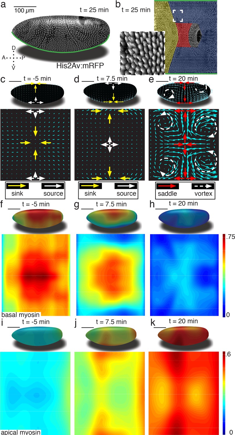
Tissue deformations of Drosophila melanogaster embryos during gastrulation, captured by three simple flow fields.
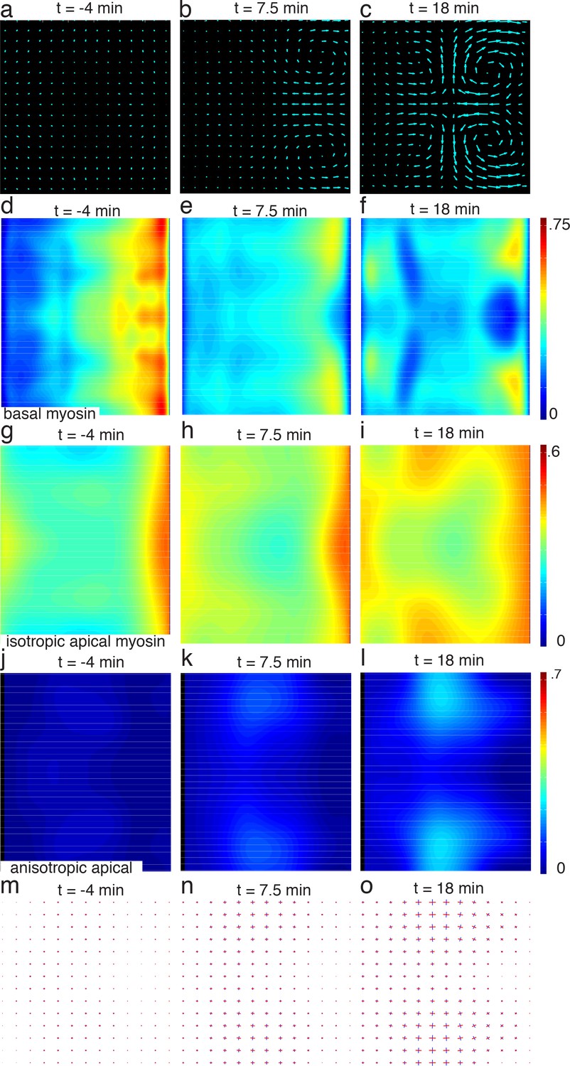
(a) Stage 7 embryo labeled with His2Av:mRFP. Anterior is to the left, dorsal up. Time is chosen such that 0 min coincides with the first occurrence of the cephalic furrow (CF). All scale bars indicate 100 µm. (b) Thin (midplane,Figure 1—figure supplement 1) layer through embryo shown in (a), with prospective head, germband and amnioserosa color-coded. Anterior is to the left, posterior to the right, dorsal is in the center and ventral is on top and bottom. Inset shows zoom into anterior germband region. (c–e) Flow field on 2D projections for representative time points of the pre-Ventral Furrow (pre-VF) phase (c), Ventral Furrow (VF) phase (d), and germband phase (GBE) (e). Cyan arrows indicate tissue flow field. Bold arrows indicate flow field topology: sinks (yellow), sources (white), saddles (red) and vortices (dashed white). Insets show flow field on corresponding 3D surface. (f–h) Normalized myosin distribution on basal cell surface corresponding to times shown in (c–e). Color code from lowest 0 to highest 1. (i–k) As (f–h) except for isotropic pool on apical cell surface.
Figure 1—figure supplement 1
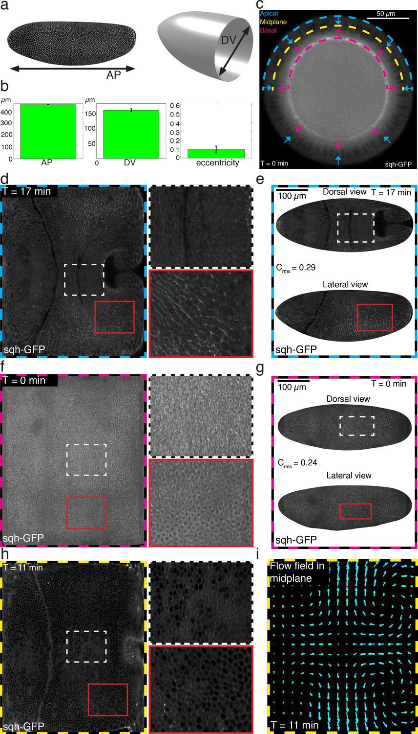
Definition of embryo shape and relevant surfaces of interest.
(a) D. melanogaster embryo shape characterized in terms of AP length, DV diameter, and eccentricity. (b) Ensemble quantification for AP length, DV diameter, and eccentricity. Error-bars indicate standard deviation. (c) DV cross section of sqh-GFP labeled embryo showing apical surface in cyan, midplane in yellow and basal surface in magenta. Arrowheads indicate normal evolution is used to relate apical and basal surfaces with the lateral surface. (d,f,h) Myosin signal on apical, basal, and midplane surface respectively as indicated by bold dashed frame. Time is indicated in each dataset with respect to cephalic furrow formation. Small insets refer to zoom on dorsal (indicated by white dashed box), and ventro-lateral region (indicated by solid red box) respectively. (e,g) Myosin signal shown in (d,f) respectively, plotted on actual apical (e) or basal (g) surface, respectively. Shown are a dorsal view on top and lateral view on the bottom. (i) The flow field used for quantitative analysis is evaluated on the midplane surface.
Figure 1—figure supplement 2

Myosin timecourse on the apical surface.
(a) Time course of Myosin visualized by sgh-GFP on apical surface, as described in Figure 1—figure supplement 1e. Root mean square contrast Crms for across the entire embryo surface is reported for each time point shown. Images have been normalized to range from 0 to 1 as described in the SI. (b) Histogram of average edge intensity. Dashed lines indicate minimum of distribution and 95th percentile determined once per dataset. Data shown are for time point 17 min (b’) As (b), except corrected for minimum and normalized to 95th percentile. (c) Histogram of edge intensities in dorsal and lateral regions, respectively.
Figure 1—figure supplement 3
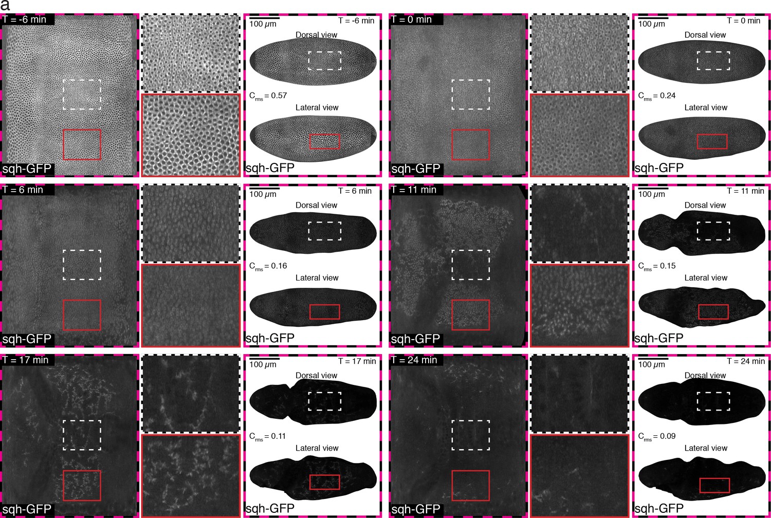
Time course of Myosin on basal surface, as described in Figure 1—figure supplement 1g.
Root mean square contrast Crms for across the entire embryo surface is reported for each time point shown. Images have been normalized to range from 0 to 1 as described in the SI.
Figure 1—figure supplement 4
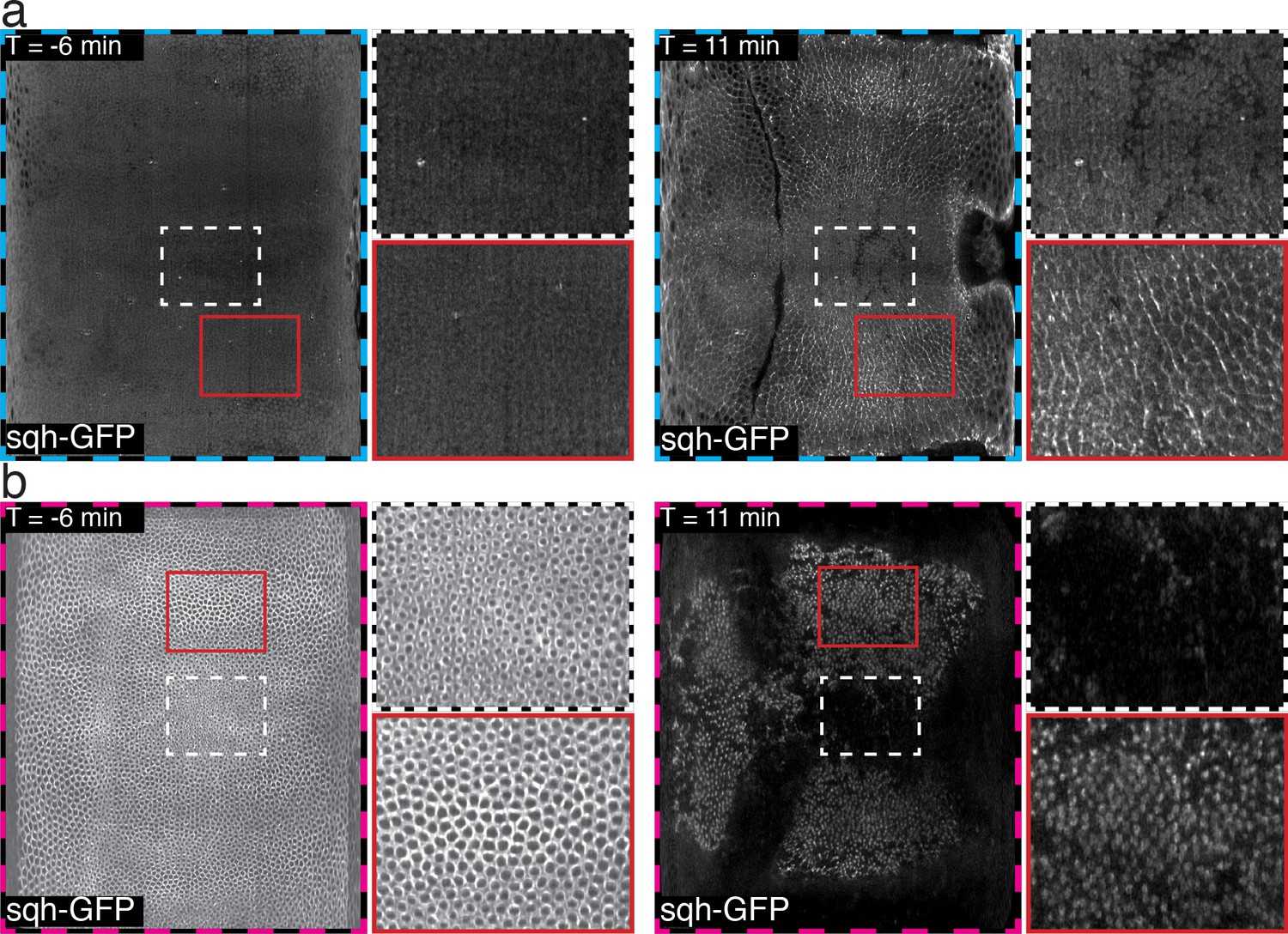
Magnified view of time course of Myosin on basal surface, as described in Figure 1—figure supplement 1e,g.
(a) apical surface. (b) basal surface. Note that in contrast to Figure 1—figure supplements 1–3, the lookup table has been adjusted in each time point separately, to enhance visualization.
Figure 1—figure supplement 5
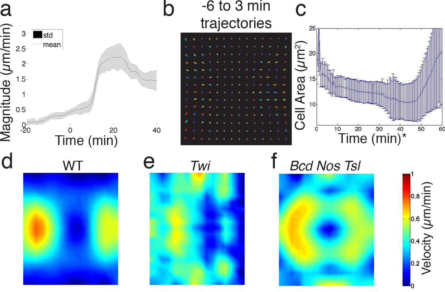
Quantitative analysis of ensemble flow field.
(a) WT ensemble averaged flow field magnitude, averaged over embryo surface. Standard deviation is across samples. (b) Flow lines obtained by integrating flow field over time, for WT embryos −6 before to 3 min past CF formation. For simplicity of visualization and each line gets a random color assigned. (c) Cell area on the dorsal side of the embryo shrinks with time (measured using confocal microscope). indicates time starts from beginning of the experiment, at a time point during cellularization. (d–f) Time average length of flow lines for WT (d), twist, and (f) bcd nos tsl embryos, at times indicated in (b).
Figure 1—figure supplement 6

Isotropic basal myosin, (as main text Figure 1g).
Dashed box indicates region used to evaluate DV asymmetry.
Figure 1—figure supplement 7

Basal myosin quantification light sheet versus confocal.
(a) Cell height as a function of embryo diameter increases monotonically until ventral furrow formation starts. (b) DV asymmetry as a function of time, measured using light sheet (black), or confocal with time calibration curve according to cell height (blue). (c) Confocal recording of DV cross-sections of embryos cut along AP axis. Colors indicate localization of myosin and dorsal visualized via antibody staining. Embryos were fixed by heat-methanol fixation (Miller et al., 1989) for staining with mouse anti-Dorsal (1:50, 7A4-S Developmental Studies Hybridoma Bank (DSHB)) and rabbit anti-myosin II (Zipper heavy chain, 1:1000, [Sokac and Wieschaus, 2008]). Secondary antibodies coupled to Alexa Fluor 488 and Alexa Fluor 564 were used at a 1:500 dilution (Invitrogen).
Figure 2 with 4 supplements
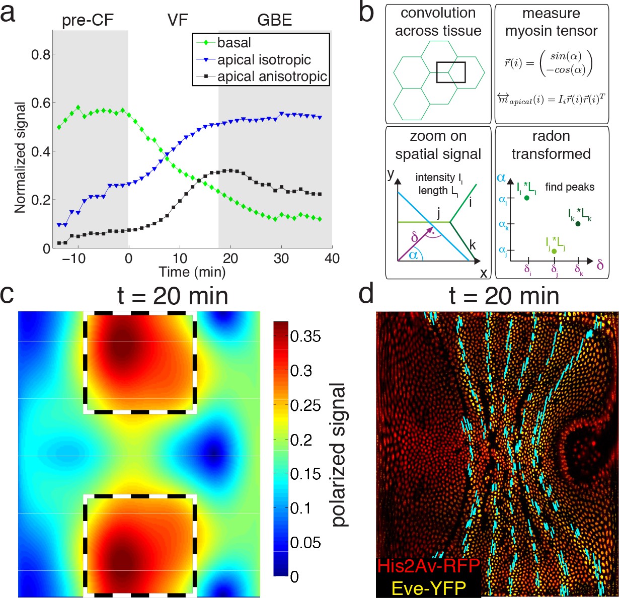
Quantitative analysis of myosin distribution and anisotropy reveals transition across pools.
(a) Normalized signal strength of basal, apical, and polarized pools over time in the lateral ectoderm (outlined as dashed box in c). First gray shaded box at t < 0 min indicates times before CF formation (pre-CF), second shaded indicates GBE. (b) Automated extraction of polarization based on images, and quantitative summary as nematic tensor. Top left box shows cell outlines in part of a tissue, and a region of interest (ROI), that moves across the tissue. Bottom left box shows zoom on spatial signal in ROI. Colors indicate potentially different intensities of lines labeled i,j,k. Average intensity and length of lines in images are denoted I and L respectively. Radon transforms integrate signal along lines (cyan) of orientation α at normal-distance δ from the origin (purple). Bottom right inset shows sketch of resulting Radon-transformed signal. Note that lines are peaks at angle α, and distance δ, of height L*I after transformation. Top right inset shows definition of unit vector with orientation of edge i. Definition of local myosin tensor (only computed on apical surface, see Figure 2—figure supplement 4) for edge i is obtained by contracting unit edge vector with itself and weighted by line average intensity. (c) Magnitude of myosin anisotropy on pullback (see SI for definition). Dashed box indicates region of interest used to compute time traces in a. (d) Axis of myosin anisotropy (in cyan) overlayed on embryo labeled with his2Av-RFP in red, and eve-YFP in yellow. For simplicity of comparison, the field is only shown along even skipped stripes. For more detailed analysis see Figure 2—figure supplement 3f.
Figure 2—figure supplement 1

Illustration of how to construct a Radon transform for an image with constant background , shown in black and foreground , shown in white (top), and resulting radon transform (bottom).
Colors indicate different lines, and the result in the radon transform is indicated as colored circle.
Figure 2—figure supplement 2
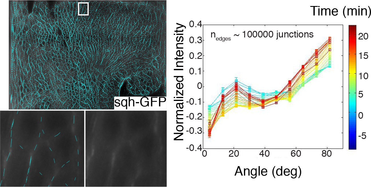
Example of edges identified with our anisotropy detection algorithm, and a magnification in a region of interest showing result in comparison with underlying raw data (left).
Time course of normalized intensity (shifted to zero mean) versus edge orientation. Color codes for time as indicated in the colorer (right).
Figure 2—figure supplement 3
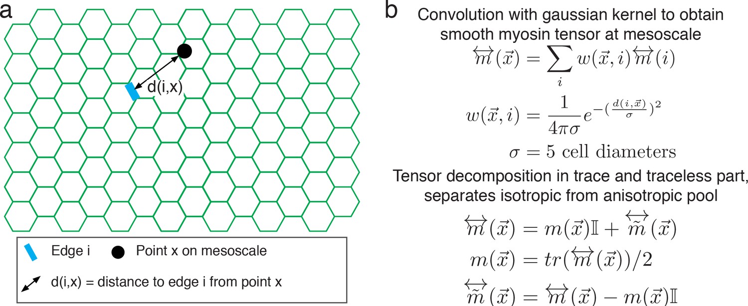
Continuous representation of myosin tensor on the mesoscale.
(a) Continuous representation of the myosin tensor. Black dot indicates coordinates on mesoscale and green cells represent the tissue. Edge i is highlighted in blue, and distance of edge i to a point x in the lattice is shown as a solid double-arrow. (b) Definition of myosin tensor on the mesoscale. Coordinates are indicated by x, edges detected by the radon transform are indicated by i. Detected edges contribute to a point by the normalized weight w(x,i), which we model as a suitably normalized Gaussian distribution. The resulting myosin tensor decomposes into a trace and a traceless part.
Figure 2—figure supplement 4
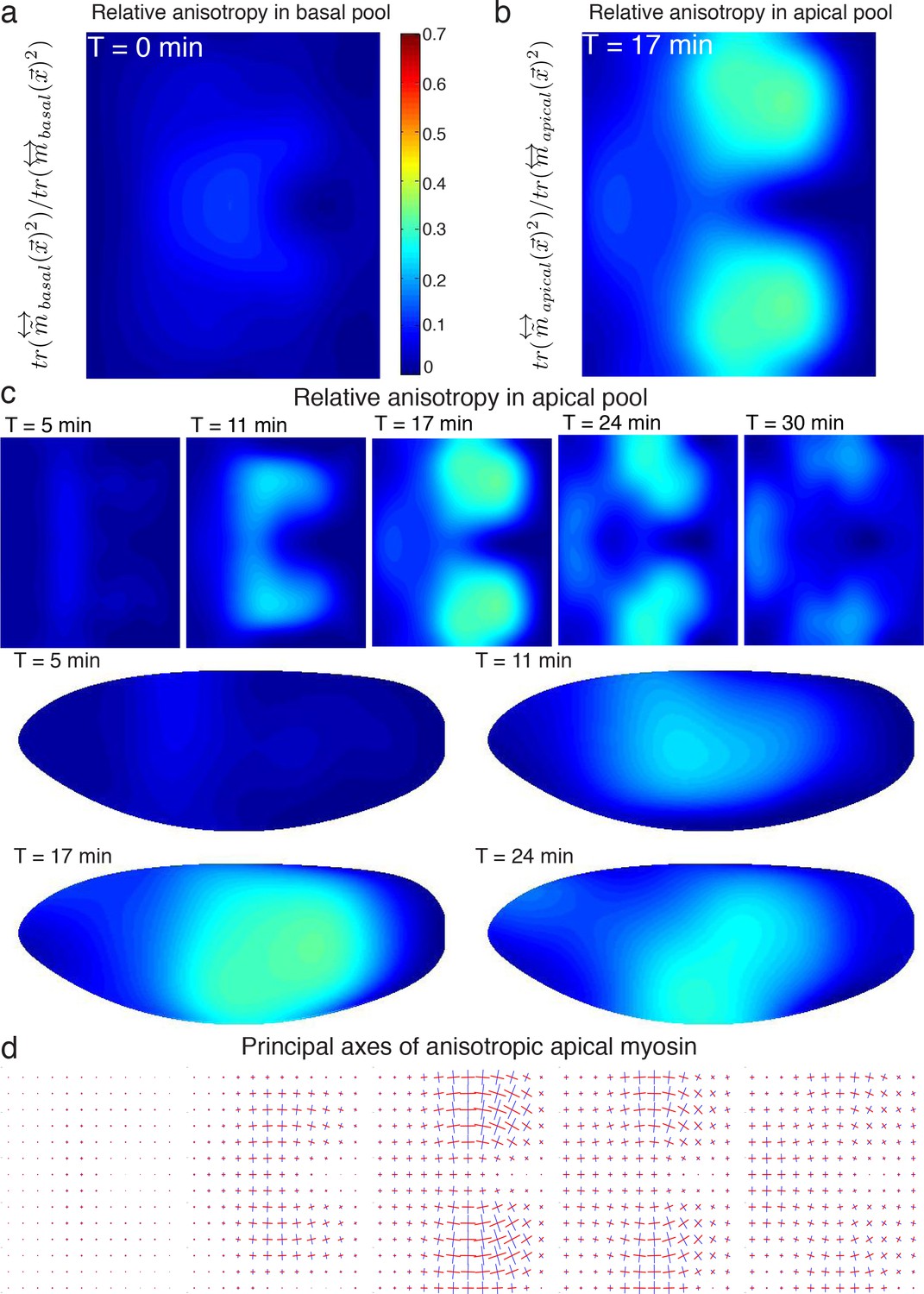
Myosin tensor on the mesoscale.
(a) Relative myosin anisotropy of basal pool, as computed by the magnitude of the traceless part over the total myosin tensor. (b) Relative myosin anisotropy of apical pool. (c) Time course of relative myosin anisotropy in the apical pool for representative time points. Definition and lookup table is the same as in (a,b). (d) Principal axes of anisotropic myosin tensor on apical surface, for times shown in (c). Major axis is shown in blue, minor in red. Magnitude is proportional to corresponding eigenvalue.
Figure 3 with 1 supplement
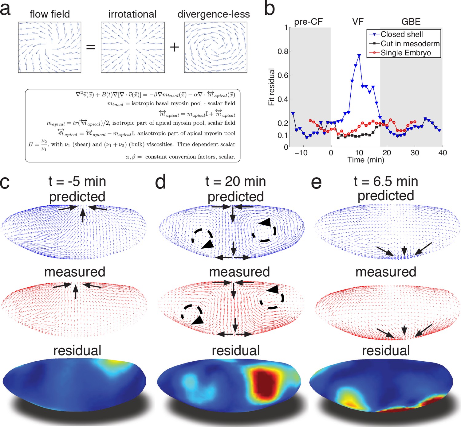
Biophysical model quantitatively predicts tissue flow based on quantitative measurements of myosin distribution.
(a) Proposed mathematical description of the flow parameterizes complex mechanics of cytoskeleton in terms of the shear ν1 and ν2 bulk effective viscosities. The flow is driven by the force proportional to the divergence of the myosin tensor (see SI) on the right-hand-side of Equation 3a. Because effective viscosity tends to suppress velocity differences of neighboring cells, the response to local forcing is felt globally, e.g. effect of a local myosin perturbation results in local as well as non-local changes of the flow field. (b) Fit residual, comparing predicted flow field with measured flow field (see SI Finite Element implementation for a detailed definition of the residual) as a function of time. Both fields are normalized for average magnitude. The average magnitude of predicted velocity field defines one of our fitting parameters. Images of the single embryo are shown in Figure 1—figure supplements 2–3 (c–e) Representative time points of morphogenetic flow: pre-CF (c), GBE (d) and VF (e). From top to bottom: spatial distribution of predicted (blue), measured (red) flow field, and residual (blue best agreement, red worst, on a scale from 0 to 1). For the case of VF flow, predictive model is modified to allow for a ‘cut’ in ventral region (see SI text, and Figure 3—figure supplement 1 for detail).
Figure 3—figure supplement 1

Finite element realization of model and parameter values.
(a) Schematic of the finite element model including the ‘cut’ used to model ventral furrow formation. Shown is a triangulation of the embryo from a ventral perspective, anterior to the left. The ‘cut’ is realized by removing all edges within the red outlined box and introducing a contractile force(shown in green) normal to the edge as boundary condition.(b) Time dependence of B, representing ratio of viscosities (see Figure 3a for detail). (c) Model summary, with explanation of temporal dependence of model parameters. Ten percent confidence intervals are indicated in brackets.
Figure 4 with 1 supplement
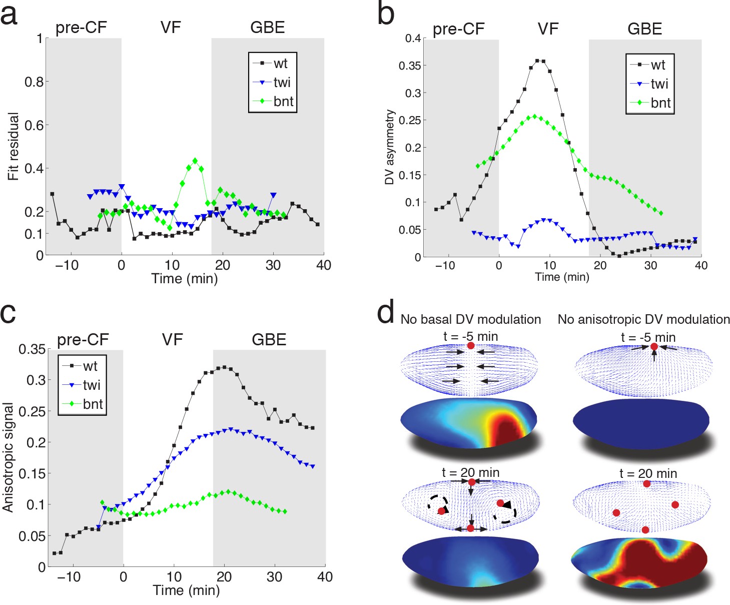
Mutant analysis reveals global modifications of myosin dynamics.
(a) Fit residual as in Figure 3b, for twi, and bcd nos tsl mutants (7, and 7 embryos in ensemble). WT is shown as reference. (b) Amplitude of basal myosin pool along DV axis for WT and mutants in (a). (c) Polarized apical myosin in mutants shown in (a) as function of time. (d) Theoretical comparison of DV constant basal pool (i.e. no gradient in DV direction) (left column), or DV constant anisotropic apical pool (i.e. no gradient in DV direction) (right column) with predicted flow based on full myosin tensor (compare to Figure 3c,d respectively). Black arrows indicate flow field topology, and red dots the fixed point from prediction based off of full myosin tensor. Model parameters are the same as previously determined for the WT (Figure 3—figure supplement 1).
Figure 4—figure supplement 1
Twist mutant flow field and myosin analysis.
(a–c). Flow field on 2D projections for representative time points. As in Figure 1c–e Cyan arrows indicate tissue flow field. (d–f) Normalized myosin distribution on basal cell surface corresponding to times shown in (a–b). Color code from lowest 0 to highest 1. (g–i) As (d–f), except for isotropic pool on apical cell surface. (j–l) Time-course of relative myosin anisotropy in the apical pool for representative time points. (m–o). Principal axes of anisotropic myosin tensor on apical surface. Color code and scale are as in Figure 2—figure supplement 3e.
Additional files
-
Transparent reporting form
- https://doi.org/10.7554/eLife.27454.019
Download links
A two-part list of links to download the article, or parts of the article, in various formats.
Downloads (link to download the article as PDF)
Open citations (links to open the citations from this article in various online reference manager services)
Cite this article (links to download the citations from this article in formats compatible with various reference manager tools)
Global morphogenetic flow is accurately predicted by the spatial distribution of myosin motors
eLife 7:e27454.
https://doi.org/10.7554/eLife.27454


