Distinct hippocampal-cortical memory representations for experiences associated with movement versus immobility
- University of California, San Francisco, United States
- Howard Hughes Medical Institute, University of California, San Francisco, United States
- University of California, Berkeley, United States
- Princeton University, United States
Figures
Figure 1 with 4 supplements

Spatial activity of CA1 place cells during movement and immobility.
(A-C) Firing properties of 4 simultaneously recorded CA1 place cells from the foraging task. Two example Immobility-Associated Place cells (IAPs) are shown in the first two columns and two example Movement-Associated Place cells (MAPs) are shown in the last two columns. (A) Occupancy normalized firing rate. Maximum rate is shown below each panel. (B) Location and speed of the animal at the time of each spike. Speed is indicated by shades of purple. Spikes during SWRs, which occur at low speeds, are shown in cyan. (C) Histogram of speed for all spikes. The histogram is stacked and the proportion of spikes during SWRs is shown in cyan. Amount of time spent in each speed category is shown in Figure 1—figure supplement 3. (D) Distribution of well specificity indices for all IAPs. (E) Median movement speed at the times of spikes for IAPs and MAPs. Even though we selected IAPs based on mean firing rate at locations of immobility, IAPs tend to only spike at low speeds rather than being generally active at all times. Wilcoxon rank-sum test: ***p<10−4. (F) Spatial coverage of IAPs and MAPs. Wilcoxon rank-sum test: ***p<10−4.
Figure 1—figure supplement 1
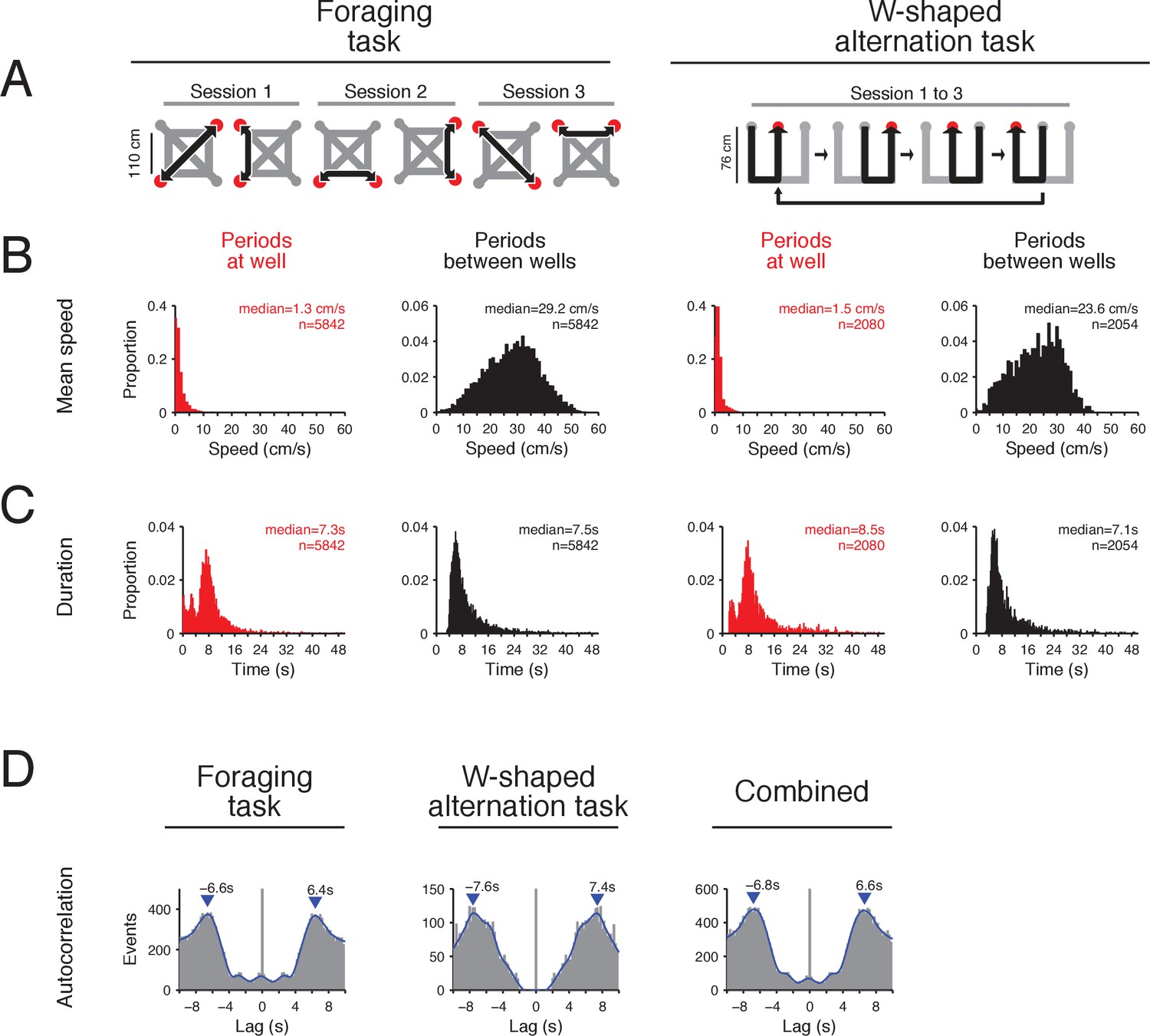
Two spatial navigation tasks with alternating periods of movement and immobility.
(A) In the foraging task (left), the maze has 4 potential reward locations (wells) located on the corners of the maze but only 2 will deliver reward for a given contingency. The animal needs to find the 2 wells that deliver reward (red circles) and alternate between the two (black arrow) to continuously receive reward. Paths (gray) connect all reward wells and the rat is free to choose any path. The locations of the rewarded wells change within session, between sessions and/or between days. The pairs of wells that are rewarded vary across sessions and the rat needs to learn the locations of the rewarded wells for every contingency by trial and error. In the W-shaped alternation task (right), an animal has to visit the wells (red circles) in the order shown by the black arrow to receive reward (Frank et al., 2000; Kim and Frank, 2009). (B) Distribution of the animal’s mean speed during periods at wells (red) and periods between wells (black) for the foraging task (left) and W-shaped alternation task (right). Subjects are immobile during periods at the well and are moving during periods between wells. Number of periods is indicated. (C) Distribution of mean durations for periods at wells (red) and periods between wells (black) for the foraging task (left) and W-shaped alternation task (right). The multiple peaks in the distribution for periods at wells correspond to different lengths of time spent at wells. In the foraging task, the two smaller peaks at 0 and 3 s for periods at wells correspond to visits for which no reward was delivered (incorrect trials) as the rats departed the well quickly after discovering the absence of reward. Number of periods is indicated. (D) Autocorrelation of times of entry into and exit from wells for the foraging task (left), the W-shaped alternation task (center) and combined data from both tasks (right). The peak of autocorrelation away from 0 is calculated from the smooth histogram (blue line) and shows periods of movement and periods of immobility are separated by 6.4–6.6 s for the foraging task, 7.4–7.6 s for the W-alternation task and 6.6–6.8 s for combined data from both tasks. These results show that on a given trial the rat transitions from immobility to movement approximately every 6.6 s. The small peak at ~3 s for the foraging task are trials on which the rat visited an unrewarded well location and quickly exited the location.
Figure 1—figure supplement 2
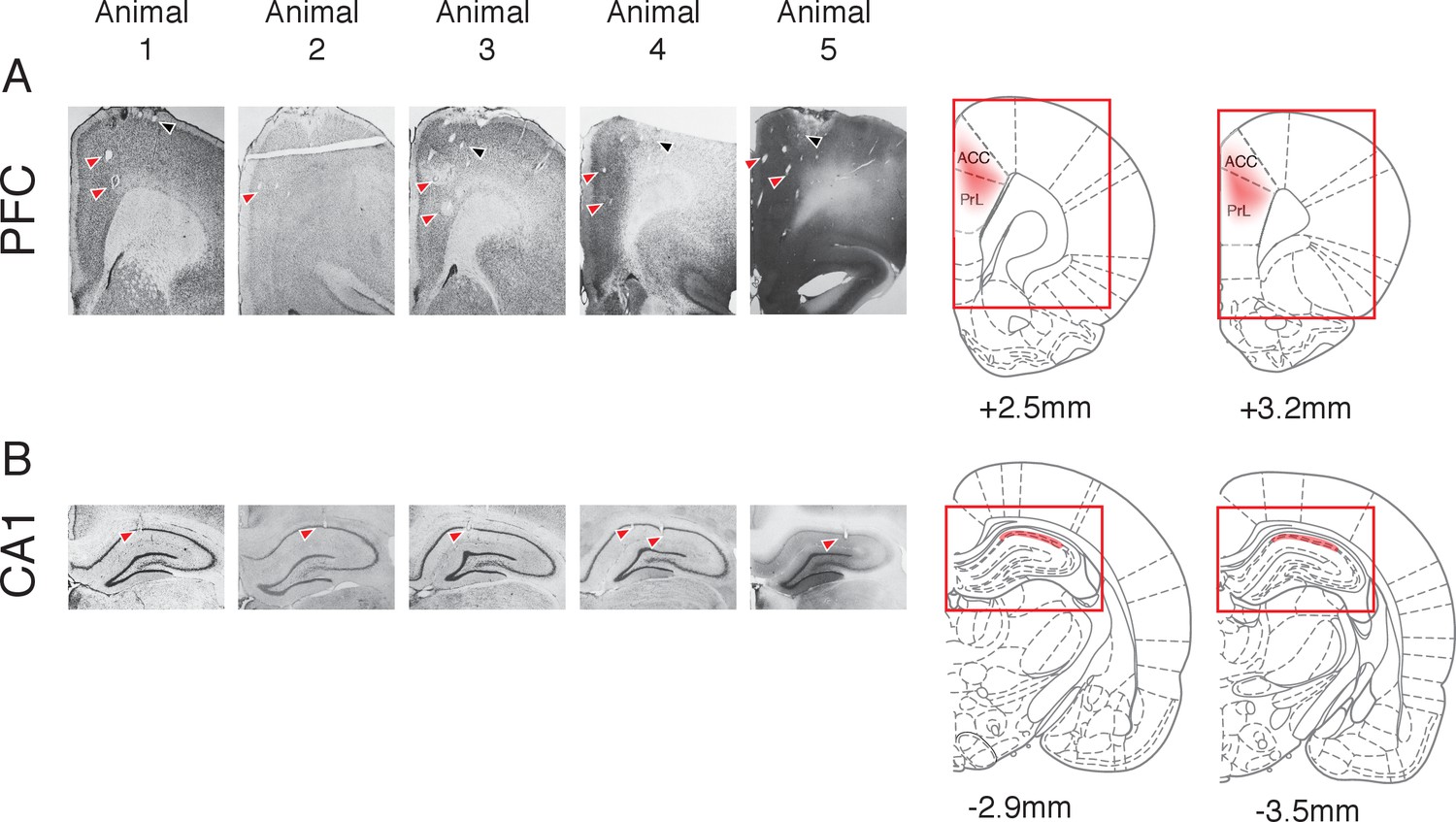
Histology of subjects that performed the foraging task.
(A) Example tetrode placement in right PFC for each subject and the estimated regions of the PFC (red) sampled across all subjects. ACC: Anterior cingulate cortex. PrL: Prelimbic cortex. (B) Example tetrode placement in right dorsal CA1 for each subject and the estimated regions of CA1 (red) sampled across all subjects. Red arrows indicate sites of electrolytic lesions corresponding to the ends of the tetrodes. Black arrows indicate locations where tetrodes passed through brain tissue. Histology for animals that performed the W-shaped alternation task has been published previously (see [Kay et al., 2016]). The anterior-posterior distance from Bregma is shown below the 2 right most panels in A and B (modified from Paxinos and Watson, 2007]).
Figure 1—figure supplement 3
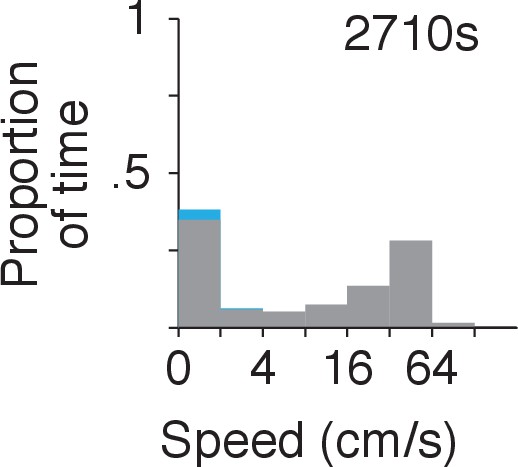
Proportion of time the animal spent in each speed category.
Period analyzed corresponds to recording sessions in Figure 1A–C. The total amount of time is indicated. The histogram is stacked and the proportion of time during SWRs is shown in cyan.
Figure 1—figure supplement 4
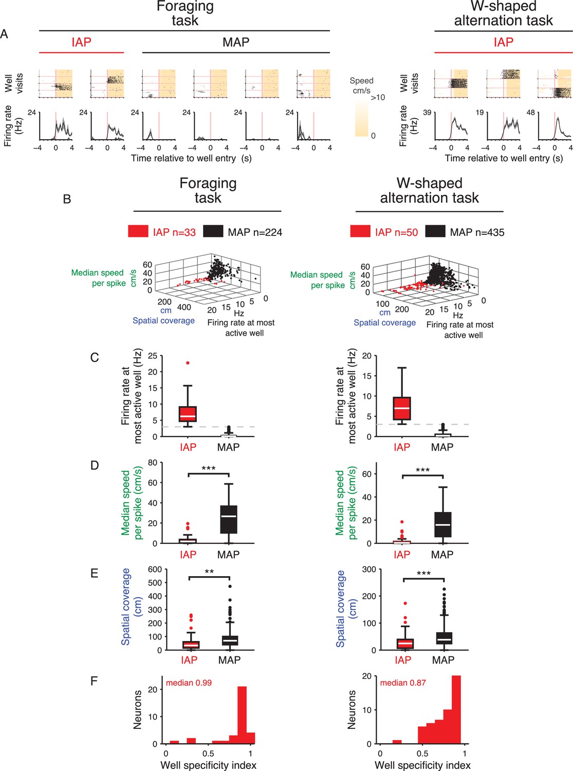
Characterization of IAPs and MAPs in each task.
(A) Spike raster of CA1 cells aligned to entry into wells (pink vertical line) for the foraging task (left) and W-alternation task (right). Cells for the foraging task (left) correspond to cells shown in Figure 1A. Upper row: Spike raster for the last 20 rewarded visits to each well (separated by horizontal pink lines). Speed is shaded in cream. Lower row: Mean firing rate of trials for each well. Note that as animals can use different paths to reach each well in the foraging task, MAPs will show activity on some trials but not others. (B) IAPs and MAPs have distinct firing properties. Cells from the foraging task are shown on left (MAP = 244, IAP = 33) and the W-alternation task on right (MAP = 435, IAP = 50). (C) Mean firing rate at the well with the highest firing rate. 3 Hz (broken line) is used as a threshold to separate IAPs and MAPs. (D) Median movement speed measured at the times of spikes from each cell. Spikes of IAPs occur at much lower speeds compared with spikes of MAPs. Wilcoxon rank-sum test: ***p<10−5. (E) Spatial coverage. IAPs have smaller place fields on path segments than MAPs. Place field size is calculated by adding all linearized spatial bins (2 cm) with a firing rate greater than 2 Hz. Wilcoxon rank-sum test: **p<0.005 and ***p<0.0005. (F) Well specificity index. Firing of IAPs is mostly specific to one location. The value (see Materials and methods) indicates how much a cell is active across all well locations. A value of 1 indicates the cell is only active at one well location while a value of 0 indicates the cell is active at all wells. IAPs in both tasks have well specificity values close to 1, which indicates firing that is specific to one well location.
Figure 2 with 2 supplements
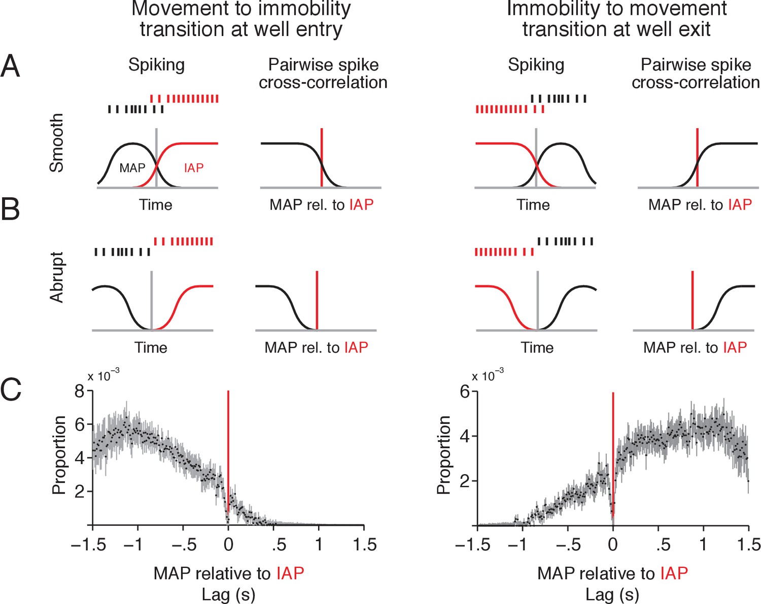
MAPs and IAPs form a continuous spatial representation during transitions between movement and immobility.
(A–B) Schematic of two scenarios for activity of MAPs and IAPs during transitions between movement and immobility as an animal enters (left column) or exits (right column) a reward well location. For a smooth transition, where spikes overlap in time between IAPs and MAPs (A), the cross-correlogram should have a tail that extends beyond 0 s lag. For an abrupt transition (B), where spikes do not overlap in time, the tail of the distribution should end at or before 0 s lag. (C) Pairwise spike cross-correlogram for spiking of MAPs relative to spiking of IAPs for spikes in a ± 1.5 s window relative to reward well location entry (left, MAP-IAP pairs n = 207) and exit (right, MAP-IAP pairs n = 217). Cross-correlation is histogrammed in 10 ms bins. Data shown as median ±1.58 × IQR divided by the square root of n, which corresponds to the notch on a box plot.
Figure 2—figure supplement 1

Spiking of MAP and IAP can be theta modulated during transitions between movement and immobility.
(A-B) Animal speed (mean ±10 SEM) relative to reward well location entry (A) and exit (B). (C-D) Autocorrelation of MAP (black line) and IAP (red line) spikes from a ± 1.5 s window centered on reward well location entry (C) and exit (D), when the animal’s speed is >4 cm/s (left) and <1 cm/s (right). Both MAP and IAP autocorrelations show peaks at intervals corresponding to theta modulation of spiking activity (0.125 s) when the animal is moving. Autocorrelations were calculated over a 1 s interval and histogrammed in 10 ms bins (mean ±SEM). Number of cells indicated in box. Cells with >100 coincident spiking events within the analysis window were included. (E-F) Pairwise spike cross-correlation over a 250 ms interval (10 ms bins) for spikes occurring within a ± 1.5 s window centered on reward well location entry (E) and exit (F). Both IAPs and MAPs can be active in the same theta cycle during the transition period between movement and immobility. MAP-IAP cell pairs are shown on the left column and MAP-MAP cell pairs are shown on the right column. Cell pairs were sorted by the peaks (white circle) of their cross-correlation relative to 0 ms lag. (G-H) Pairwise spike cross-correlation on a trial timescale (6.6 s) for all spikes outside of SWRs during the task. The cross-correlation was histogrammed into 10 ms bins and smoothed with a Gaussian kernel (σ = 150 ms, 900 ms sliding window). Cell pairs are shown in the same order as (E-F). MAP-IAP cell pairs are shown on the left column and MAP-MAP cell pairs are shown on the right column. Peaks in cross-correlations are indicated with white circles. (I-J) Scatter and correlation between the peaks in (E-F) and (G-H). Cross-correlation peaks on a theta time scale are significantly correlated with cross-correlation peaks on a behavioral time scale over seconds.
Figure 2—figure supplement 2
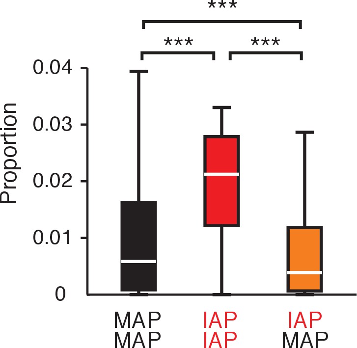
Lower proportion of coincident spikes between IAP and MAP pairs compared with MAP pairs or IAP pairs.
The proportion of spike pairs in a pairwise spike cross-correlation occurring within ±50 ms out of all spike pairs occurring within a 6.6 s window (±3.3 s), which corresponds to a typical movement or immobility period. MAP-MAP (black): n = 2062. IAP-IAP (red): n = 26. MAP-IAP (orange): n = 497. Wilcoxon rank-sum test: ***p<10−4.
Figure 3 with 3 supplements
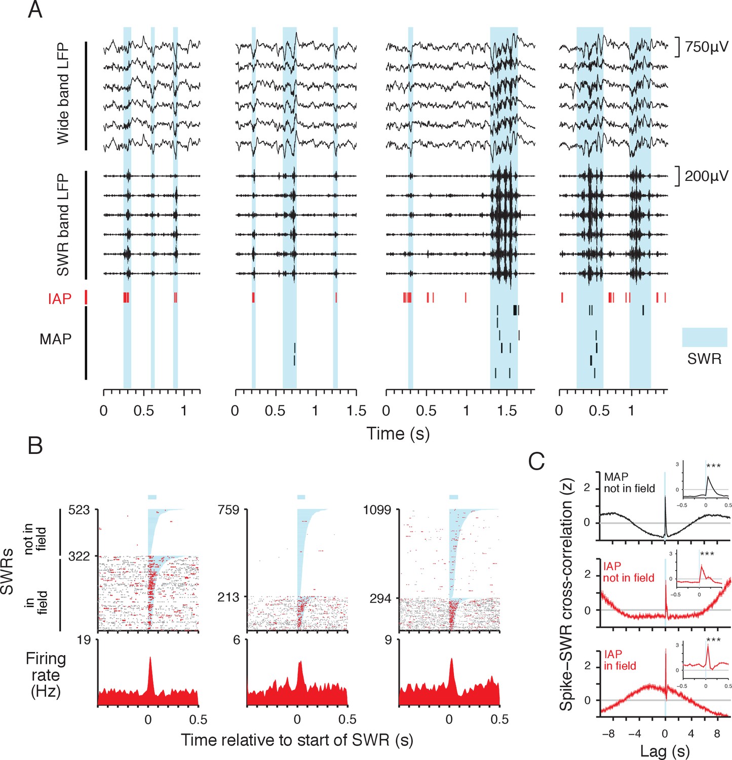
IAPs are reactivated during SWRs.
(A) Example local field potential (LFP) and place cell spiking during SWRs (cyan). Wide band LFP (1–400 Hz) and SWR band LFP (150–250 Hz) traces from 6 simultaneously recorded sites in CA1 are shown. IAP spikes are shown in red and MAP spikes are shown in black. The four examples correspond to immobile periods at wells in the foraging task. All examples are from the same day. (B) Spiking activity of three IAPs aligned to the start of SWRs. Spikes within the duration of SWRs are colored red and spikes outside of SWRs are colored grey. In field events are SWRs occurring at the reward well where the IAP has a place field. Not in field events occur at other reward wells. The orders of in field and not in field SWRs are sorted separately by SWR duration (shaded cyan, mean duration indicated by bar above spike raster). Bottom: firing rate histogram shows mean firing rate across all SWRs. Leftmost example is the IAP shown in (A). (C) Normalized cross-correlation (mean ±SEM, 50 ms bins) of MAP (black, n = 589) and IAP (red, n = 77) spiking relative to start of SWRs (cyan line). For MAPs, SWRs that do not occur within the cells' place fields and are referred to as not in field events. For IAPs, the cross-correlation of spikes and not in field SWRs is shown in middle panel, and the cross-correlation of spikes and in field SWRs is shown in lower panel. Lag refers to time relative to the start of SWR events. Inset shows the cross-correlation in a 1 s window centered at 0 s lag. For in and not in field events, both IAPs and MAPs show significant increases in activity aligned to the start of SWRs (250 ms pre vs. 250 ms post SWR start, Wilcoxon rank-sum test: ***p<10−4). We note that SWRs tend to occur during immobility, thus IAP activity is higher within seconds around the time of in field SWRs compared with MAPs and not in field SWRs.
Figure 3—figure supplement 1
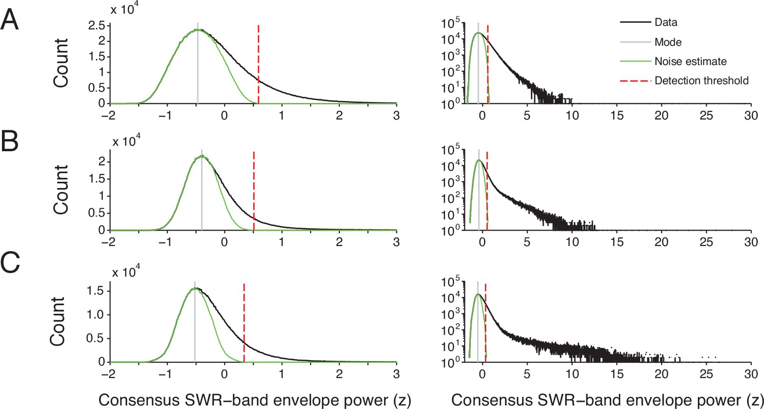
SWR detection threshold determination.
(A-C) The consensus SWR-band envelope power distribution from one recording day for 3 subjects. The SWR-band is sampled at 1.5 kHz. Left column shows the distribution of normalized SWR-band envelope power (black line) from −2 to 3 standard deviations from the mean (z-score units). The right column shows the distribution up to 30 z, with counts on a log scale. Only times when speed is <4 cm/s were included. The power distribution varied between days and animals and an arbitrary, fixed threshold for detecting SWRs will result in different levels of sensitivity for each dataset. To determine an appropriate SWR threshold, we assumed the distribution has a low-power noise component and a high-power signal component. To estimate the noise component, we created a symmetrical distribution (green line) by mirroring the left hand side of histogram at the mode (gray line) of the entire power distribution. The detection threshold (broken red line) is the 99.99th percentile of the estimated noise distribution. See Methods.
Figure 3—figure supplement 2

Baseline spiking-SWR cross-correlation for SWRs that occurred within the place field of IAPs.
Red: normalized spike-SWR cross-correlation between IAP spikes and in field SWRs. Gray: spike-SWR cross-correlation when IAP-SWR times were randomly shifted by up to ±500 ms. Inset: close up of cross-correlation for ±0.5 s. 50 ms bins.
Figure 3—figure supplement 3
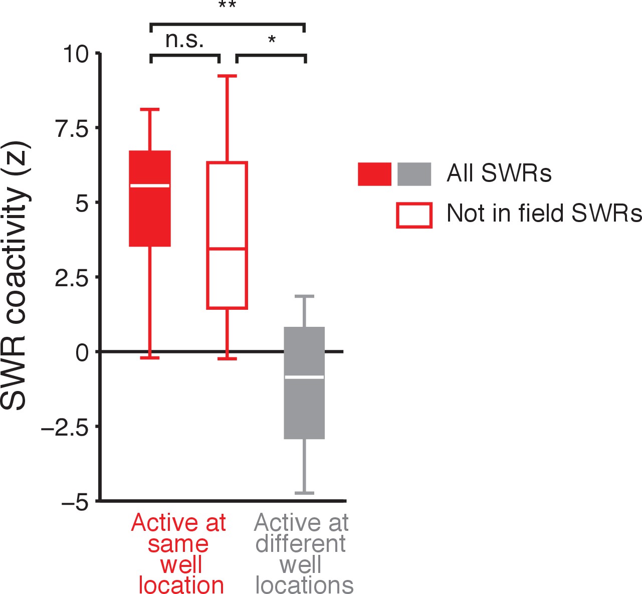
SWR coactivity for IAPs.
Boxplot of IAP coactivity for IAP pairs active at the same well location (red) or pairs active at different well locations (gray). The coactivity for all SWRs is shown by solid boxes and the coactivity for SWRs that occurred outside the IAPs’ place fields is shown by the empty box. IAPs active at same well location: all SWRs (n = 12) and not in field SWRs (n = 11). IAPs active at different well locations: all SWRs (n = 14). Kruskall-Wallis test: n.s. not significant, *p<0.05 and **p<0.005.
Figure 4 with 9 supplements
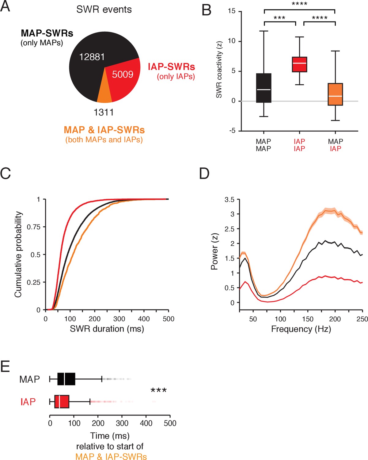
Separate SWR reactivation of IAPs and MAPs.
(A) Count of SWRs containing MAPs and IAPs. (B) Coactivity during SWRs for MAP-MAP pairs (black, n = 1015) and IAP-IAP pairs (red, n = 13) is higher than IAP-MAP pairs (orange, n = 138). Wilcoxon rank-sum test: ***p<10−3 and ****p<10−4. Data from both tasks are combined. Only cell pairs that are active within half the duration of a typical trial (peak cross-correlation <3.3 s) were included. This time is derived from the time course of bouts of movement and immobility in the task (Figure 1—figure supplement 1D). Outliers are not shown. (C) Cumulative distribution of durations for SWR events in (A). Kolmogorov-Smirnov test: p<10−4 for all pairwise comparisons between groups. (D) LFP spectral power (mean and 95% confidence of the mean) in a 100 ms window aligned to the start of SWRs normalized to all times in a task session. The mean of spectral power between 150–250 Hz is significantly different between groups. Wilcoxon rank-sum test: all pairwise comparisons p<10−4. (E) Time of MAP (black) and IAP (red) spiking relative to the start of MAP and IAP-SWRs. IAPs spike earlier than MAPs during MAP and IAP-SWRs. Wilcoxon rank-sum test: ***p<10−4.
Figure 4—figure supplement 1
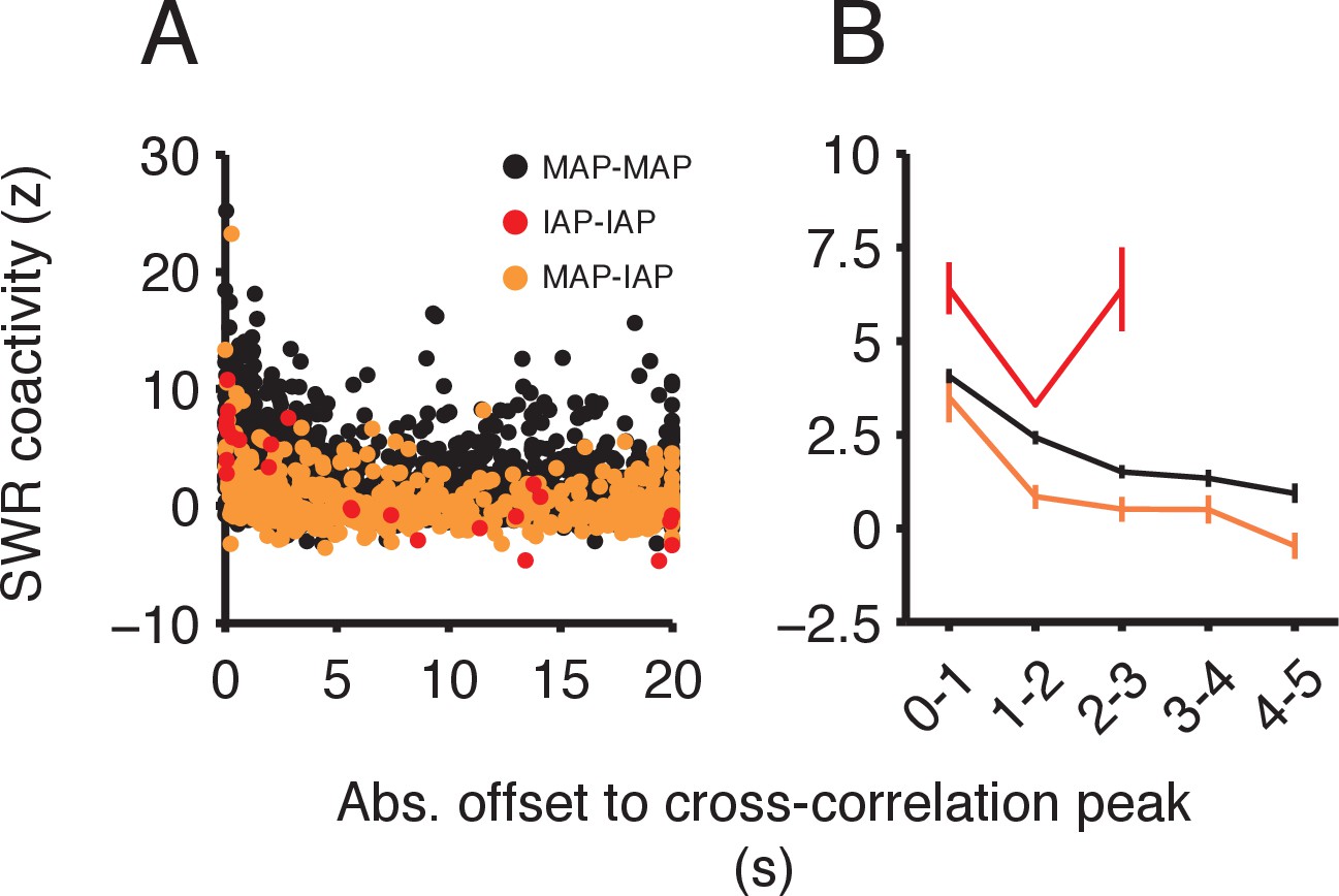
Control for the effect of temporal proximity of spiking activity on SWR coactivity.
(A) Scatter of SWR coactivity and absolute offset to cross-correlation peak for spiking outside of SWRs. MAP-MAP cell pairs (n = 2204), IAP-IAP cell pairs (n = 26) and MAP-IAP cell pairs (n = 521). (B) SWR coactivity (mean ±SEM) for offset to cross-correlation peak binned into 1 s intervals for offsets between 0–5 s. Even when matched for the offset to the cross-correlation peak, MAP-MAP pairs showed, on average, higher SWR coactivity than MAP-IAP pairs. This difference was significant for each offset bin above 1 s. Wilcoxon rank-sum tests: 1–2 s P<10−3, 2–3 s P<0.05, 3–4 s P<0.05 and 4–5 s p<0.005. The smaller, non-significant difference for offsets <1 s could contribute to associations between a subset of MAP and IAP pairs, and thus may explain the small number of SWRs where both MAPs and IAPs were active.
Figure 4—figure supplement 2

Control for the effects of spatial proximity of spiking activity on SWR coactivity.
(A) Scatter of SWR coactivity and distance between place field peaks. MAP-MAP cell pairs (n = 2203), IAP-IAP cell pairs (n = 26) and MAP-IAP cell pairs (n = 521). (B) SWR coactivity (mean ±SEM) for cells pairs with distances between place field peaks in the range 0-1 m binned into 0.25 m intervals. Across all distances, MAP-MAP pairs showed stronger coactivity than comparable MAP-IAP pairs. Wilcoxon rank-sum tests: 0–0.25 s P<10−4, 0.25–0.5 s P<10−4, 0.5–0.75 s P<10−4 and 0.75–1 s P<0.05. (C) Boxplot of SWR coactivity for cell pairs in each group with place field peaks <0.5 m. MAP-MAP (n = 1056), IAP-IAP (n = 18) and MAP-IAP cell pairs (n = 211). Outliers are not shown. Kruskall-Wallis test: ***p<10−3 and ****p<10−4. We chose not use distance between place field peaks as a way to select cell pairs for the SWR coactivity analysis due to the geometry of our task environments. We reasoned that in environments that restrict the animal’s movement to linear trajectories, such as a linear track, distance between place field peaks is more likely to be directly related to whether a pair of place cells will be reactivated together since the animal is forced to traverse the cells’ place fields sequentially. However, our foraging task has a spatial geometry with multiple intersections. Place cells with nearby place fields may not necessarily be visited sequentially depending the route choice of the animal. Temporal proximity is thus a better covariate when comparing SWR coactivity in our tasks.
Figure 4—figure supplement 3
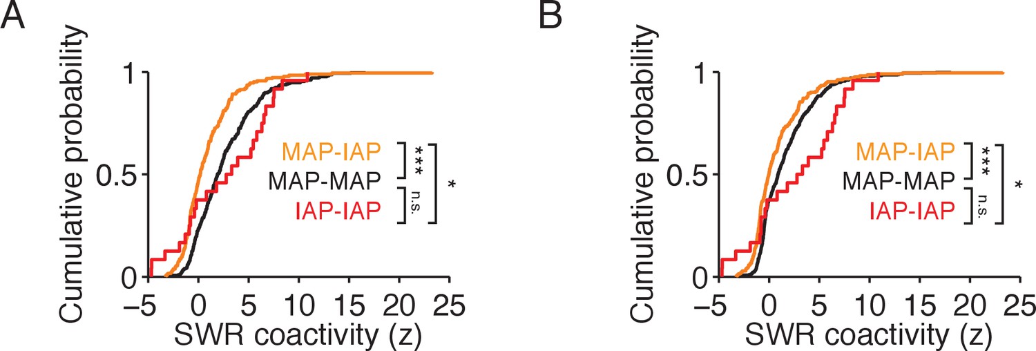
MAP and IAP pairs with temporal spiking overlap during movement and immobility transitions show lower SWR coactivity than MAP-MAP and IAP-IAP pairs.
(A) Cumulative distribution of SWR coactivity for cell pairs with temporal spiking overlap during a ± 1.5 s window centered on reward well location entry. MAP-MAP SWR coactivity (black, n = 333). MAP-IAP SWR coactivity (orange, n = 207). IAP-IAP SWR coactivity (red, n = 24). (B) Cumulative distribution of SWR coactivity for cell pairs with temporal spiking overlap during a ± 1.5 s window centered on reward well location exit. MAP-MAP SWR coactivity (black, n = 512). MAP-IAP SWR coactivity (orange, n = 217). IAP-IAP SWR coactivity (red, n = 24). Wilcoxon rank-sum test: *p<0.05 and ***p<10−4.
Figure 4—figure supplement 4
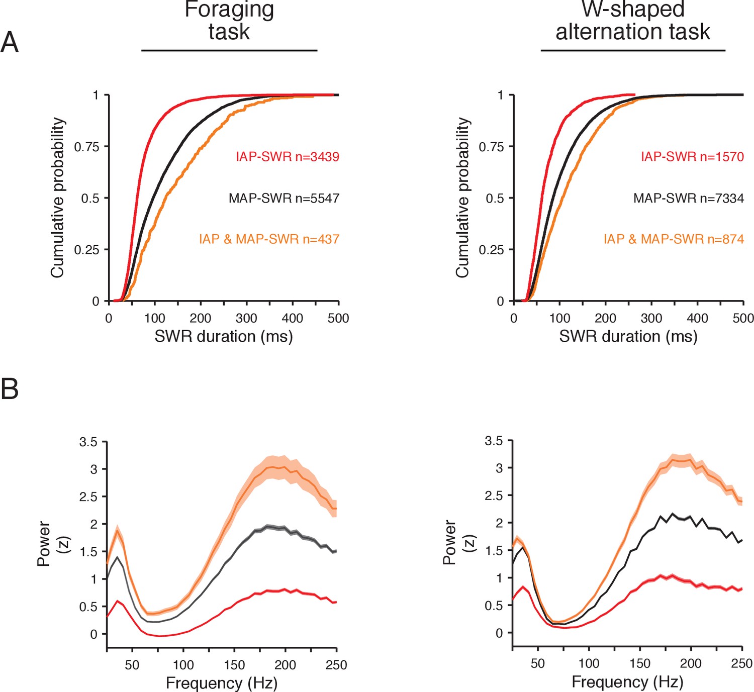
Spectrotemporal properties of SWR groups are consistent between the foraging and the W-shaped alternation task.
(A) Cumulative distribution of SWR durations for the foraging task (left) and the W-shaped alternation task (right). The number of events for each category is indicated. (B) LFP spectral power (mean and 95% confidence interval of the mean) in a 100 ms window aligned to the start of SWRs normalized to all times in a task session for the foraging task (left) and the W-shaped alternation task (right).
Figure 4—figure supplement 5
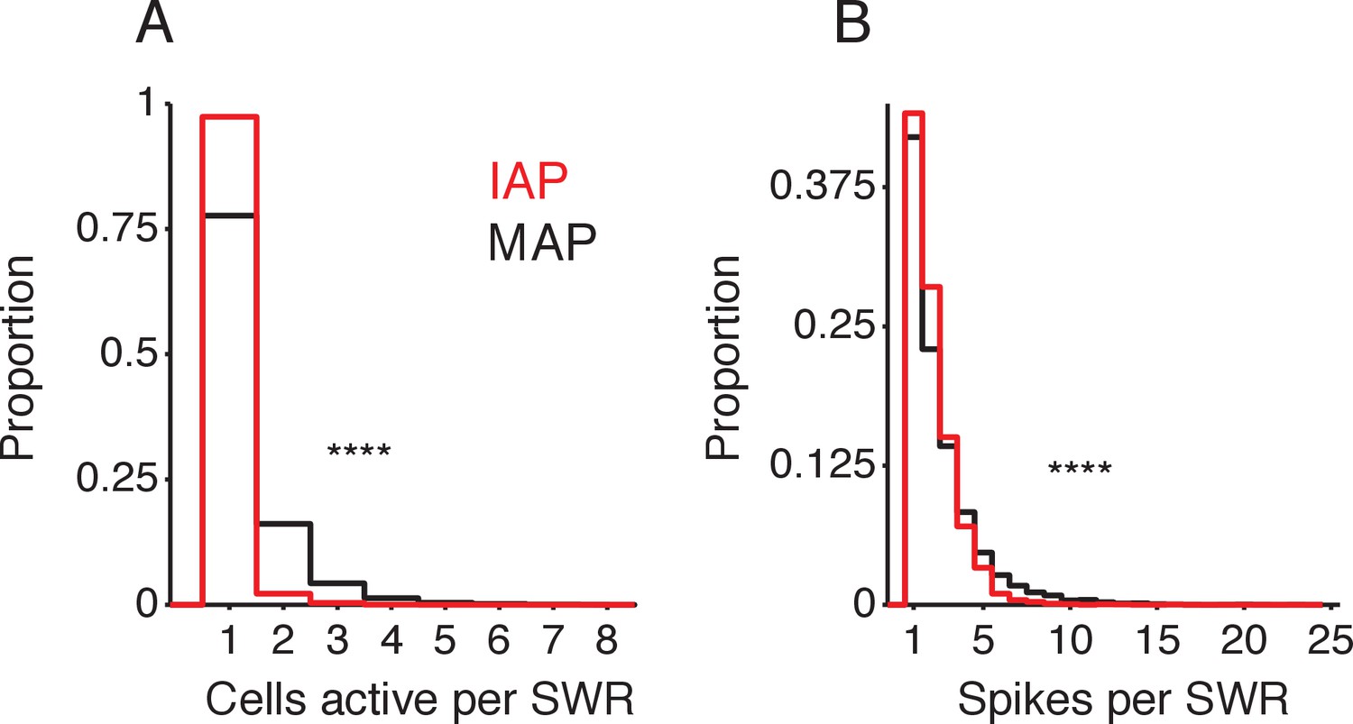
Cell and spike count during SWRs.
(A) Cells active per SWR. IAP mean = 1.03 and MAP mean = 1.31. (B) Spikes per SWR. IAP mean = 2.04 and MAP mean = 2.49. Wilcoxon rank-sum test: ****p<10−4.
Figure 4—figure supplement 6
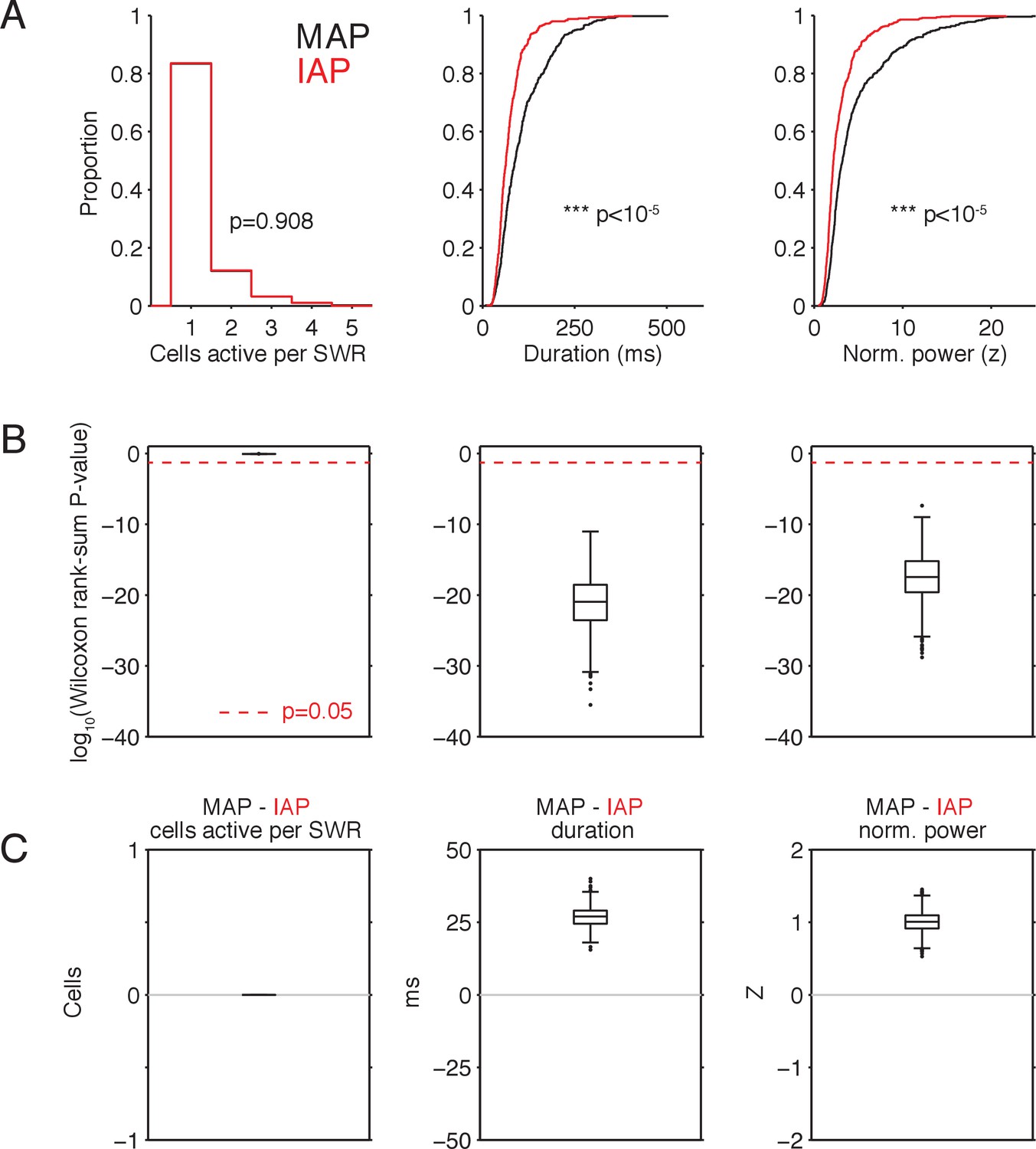
Subsample to match cells active per SWR.
(A) Example subsample to match the distribution of cells active per SWR between MAP- and IAP-SWRs (probability distribution, left). Their corresponding durations (cumulative probability distribution, center) and normalized SWR power (cumulative probability distribution, right) were compared. For the subsample, 500 values were drawn with replacement from each population. Wilcoxon rank-sum P-values are indicated. (B) Boxplots of Wilcoxon rank-sum test P-values for 1000 subsamples. Each column corresponds to comparisons in A. Broken line indicates p=0.05. SWR duration and power remain significantly different after matching for cells active per SWR. (C) Boxplots of differences in median values between the MAP- and the IAP-SWR comparisons for the 1000 subsamples in B. MAP-SWRs remain longer in duration and higher in power after matching for cells active per SWR.
Figure 4—figure supplement 7
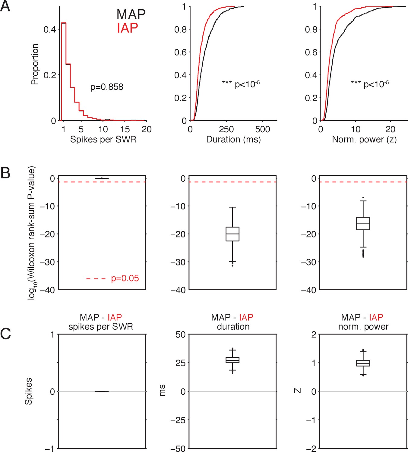
Subsample to match spikes per SWR.
(A) Example subsample to match the distribution of spikes per SWR between MAP- and IAP-SWRs (probability distribution, left). Their corresponding durations (cumulative probability distribution, center) and normalized SWR power (cumulative probability distribution, right) were compared. For the subsample, 500 values were drawn with replacement from each population. Wilcoxon rank-sum P-values are indicated. (B) Boxplots of Wilcoxon rank-sum test P-values for 1000 subsamples. Each column corresponds to comparisons in A. Broken line indicates p=0.05. SWR duration and power remain significantly different after matching for spikes per SWR. (C) Boxplots of differences in median values between the MAP- and the IAP-SWR comparisons for the 1000 subsamples in B. MAP-SWRs remain longer in duration and higher in power after matching for spikes per SWR.
Figure 4—figure supplement 8
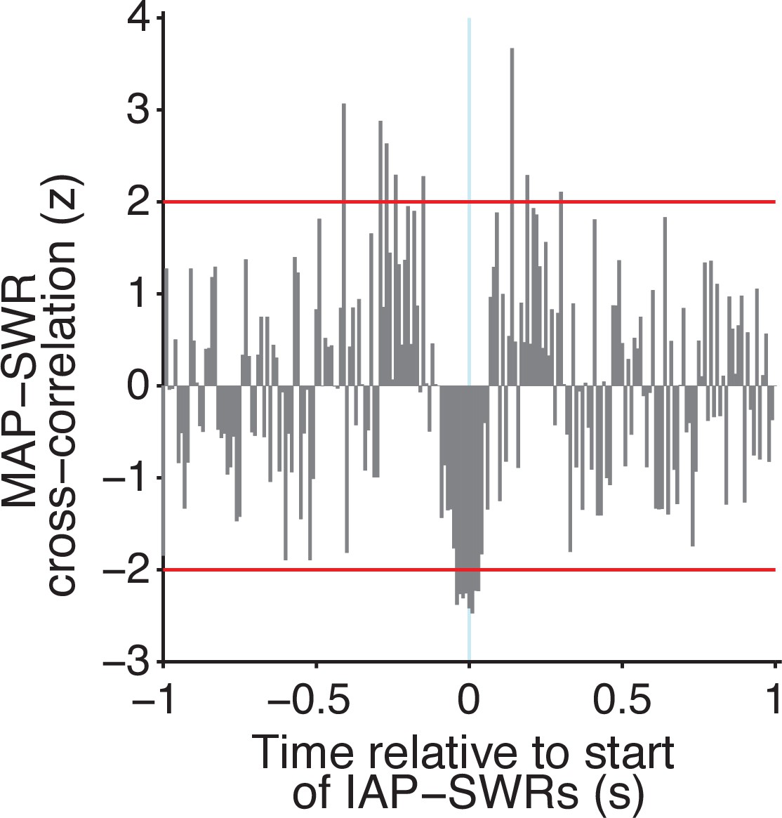
Cross-correlation between MAP- and IAP-SWRs.
The cross-correlation for each 10 ms bin was normalized to 1000 baseline control cross-correlations each generated by randomly shifting the times of MAP-SWRs by ±0–1 s. The significant dip in cross-correlation around 0 s is due to the duration of SWRs. Redlines mark ±2 z.
Figure 4—figure supplement 9

IAPs spike earlier than MAPs during MAP & IAP-SWRs after matching SWR durations.
(A) The duration of MAP & IAP-SWRs were resampled to match the distribution of SWR lengths from which MAP (black) and IAP (red) spikes were selected. (B) Timing of MAP (black) and IAP (red) spiking relative to the start of SWRs after matching the distribution of SWR durations. Wilcoxon rank-sum test: ***p<10−4.
Figure 5 with 2 supplements
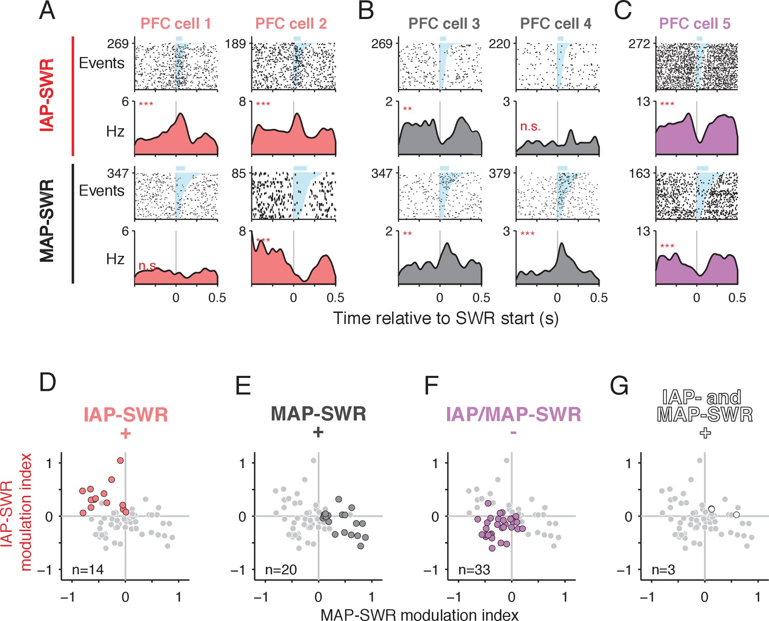
PFC modulation during SWRs distinguishes between MAP- and IAP- SWRs.
(A-C) PFC spiking activity aligned to SWRs. Spike raster (first and third rows, number of SWR events shown on y axis) and mean firing rate (second and fourth rows) for each cell are shown. Upper two rows: firing aligned to IAP-SWRs. Lower two rows: firing aligned to MAP-SWRs. SWRs are sorted by length (shaded in cyan, mean duration shown by blue bar above raster). n.s. not significant, **p<0.005 and ***p<0.0005 using a circular permutation test (Materials and methods). (A) Two example cells showing a significant increase in firing during IAP-SWRs but no change (cell 1) or a significant decrease in firing (cell 2) during MAP-SWRs. (B) Two example cells showing a significant increase in firing around MAP-SWRs but no change (cell 3) or a significant decrease in firing (cell 4) during IAP-SWRs. (C) Example cell showing significant decreases in firing during both IAP-SWRs and MAP-SWRs. (D-G) PFC units showing significant changes in activity during SWRs (n = 70, gray circles) classified into one of four groups (colored circles), based on the significance of their modulation indices for IAP-SWRs (y axis) and MAP-SWRs (x axis). The gray circles are repeated in each panel and the colored circles highlight cells belonging to each group (cell count shown in each panel). (D) Significantly excited only during IAP-SWRs (IAP-SWR+) (observed = 14, expected = 18, Binomial test n.s.). See Materials and methods for calculation of expected values. (E) Significantly excited only during MAP-SWRs (MAP-SWR+) (observed = 20, expected = 18, Binomial test n.s.). (F) Significantly inhibited during either or both IAP-SWRs and MAP-SWRs (IAP/MAP-SWR-) (observed = 33, expected = 26, Binomial test: n.s.). (G)Significantly excited during both IAP-SWRs and MAP-SWRs (IAP- and MAP-SWR+) (observed = 3, expected = 9, Binomial test: p<0.05). Fewer than the expected number of cells was observed in this group.
Figure 5—figure supplement 1
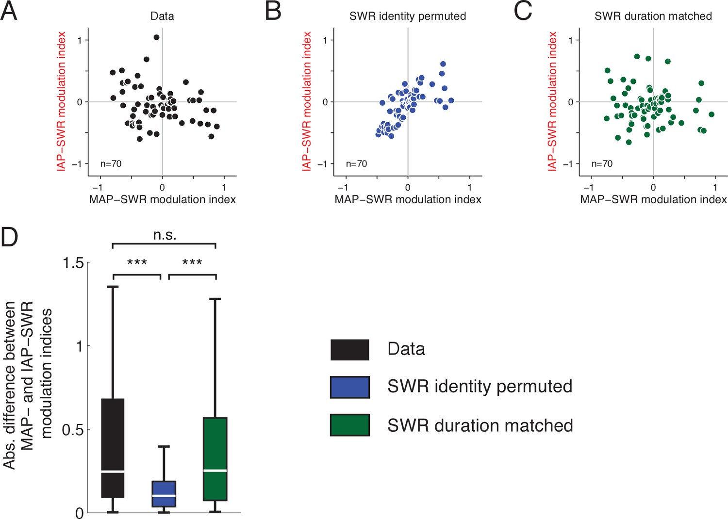
PFC modulation patterns distinguish between the identity of IAP- and MAP-SWRs and not differences in SWR duration.
(A) PFC modulation during MAP-SWRs (x axis) and IAP-SWRs (y axis). The units shown are those with significant modulation to either or both MAP- and IAP-SWRs and are the same as those in Figure 5D–G. (B) PFC modulation of each unit in A after permuting the identity of SWRs. (C) PFC modulation of each unit in A after resampling SWR events to match the distributions of SWR durations for MAP-SWRs and IAP-SWRs. For each unit from the original datasets, 250 SWR events were randomly drawn with replacement before recalculating the SWR modulation indices. (D) The difference between MAP-SWR and IAP-SWR modulation indices was significantly decreased when the identities of SWRs are shuffled (blue) but remained similar to the original data after SWR durations wee matched (green). Wilcoxon rank-sum test: ***P<10-3. PFC modulation during MAP-SWRs and IAP-SWRs were distinct and wass not due to different durations of MAP- and IAP-SWRs.
Figure 5—figure supplement 2
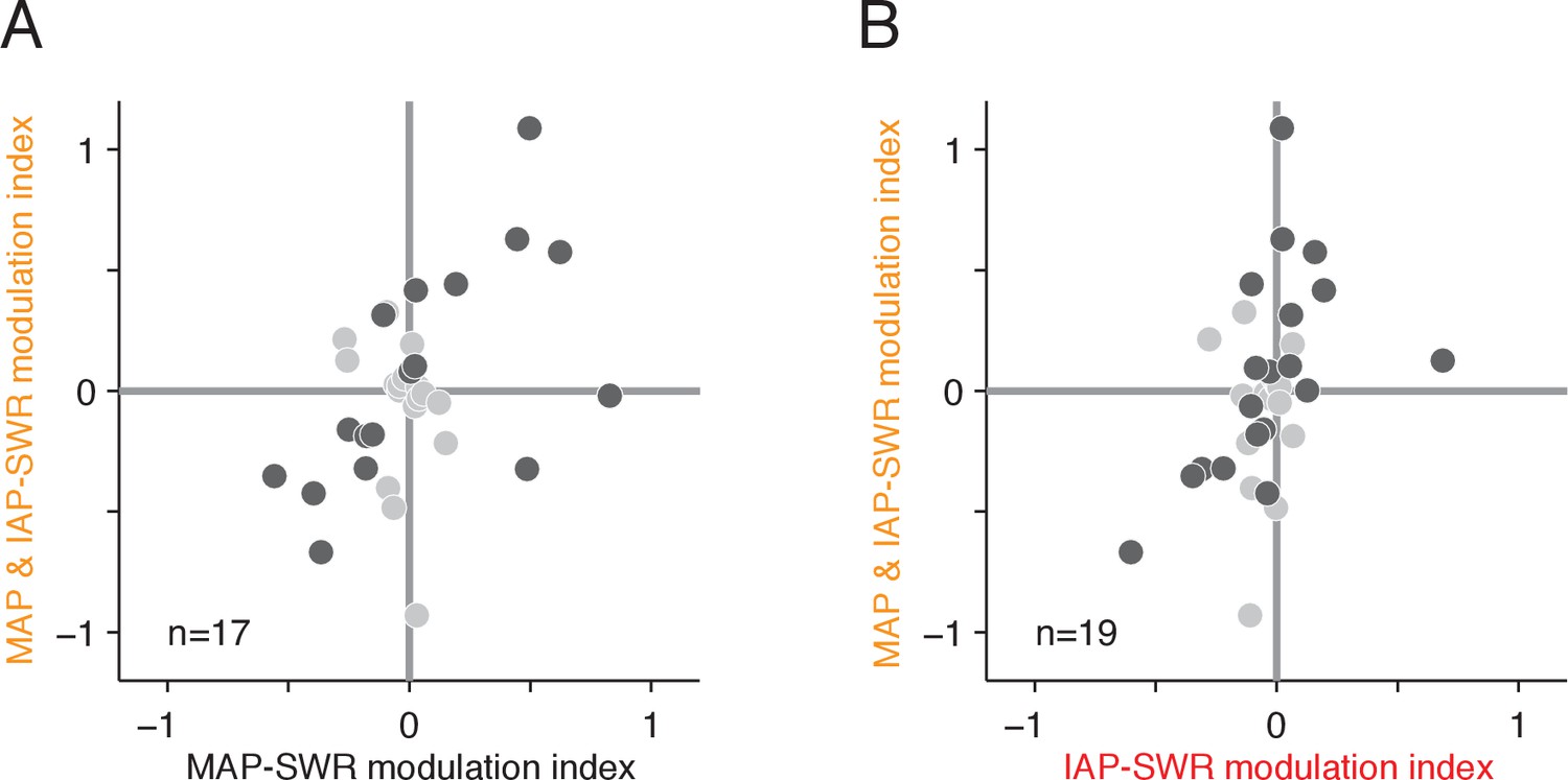
PFC modulation patterns during MAP and IAP-SWRs.
(A) MAP & IAP-SWR modulation versus MAP-SWR modulation. Black circles: cells with significant modulation (p<0.05) during at least one type of SWR (n = 17). Gray circles: not significantly modulated. (B) MAP & IAP-SWR modulation versus IAP-SWR modulation. Black circles: cells with significant modulation (p<0.05) during at least one type of SWR (n = 19). Gray circles: not significantly modulated.
Figure 6 with 2 supplements
PFC SWR modulation reflects task firing properties.
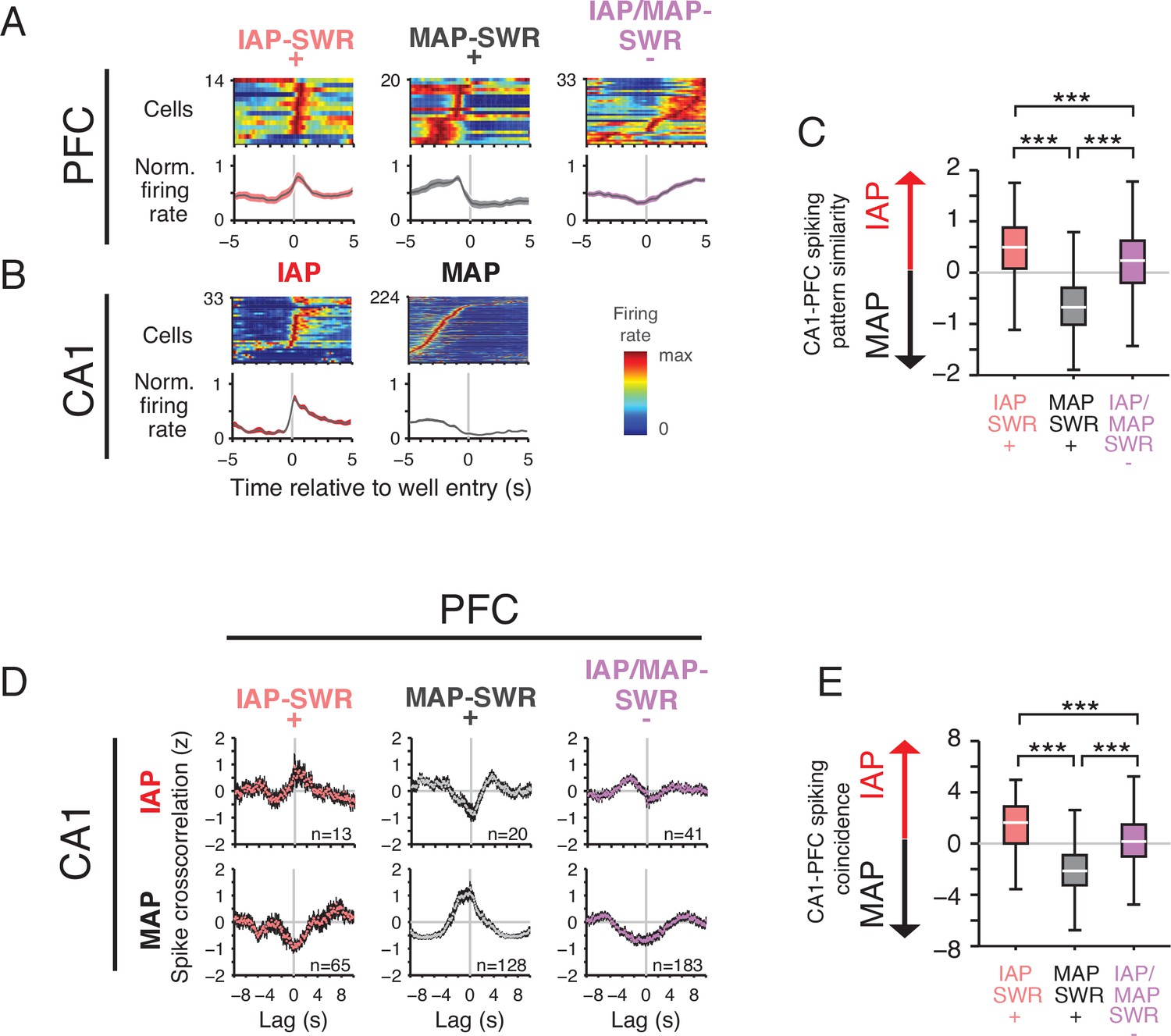
(A) Mean firing rate for significantly SWR modulated PFC units aligned to reward well entry. PFC units are grouped by their participation in IAP-SWRs and MAP-SWRs (Figure 5D). Top row: firing rate of each cell in each group normalized to maximum firing rate in the −5 s to 5 s time window. Bottom row: mean normalized firing rate (±SEM) for all cells in each group. (B) Mean firing rate for CA1 cells aligned to well entry. Top row: firing rate of each cell in each group normalized to maximum firing rate in the −5 s to 5 s time window. Bottom row: mean normalized firing rate (±SEM) for all cells in each group. (C) Firing pattern similarity index for each PFC cell group. The similarity index is the pairwise difference in correlation value between the firing pattern correlations for all possible PFC-CA1 IAP and all possible PFC-CA1 MAP cell pairs. A value greater than 0 indicates similarity to IAP firing whereas a value less than 0 indicates similarity to MAP firing. Wilcoxon rank-sum test: ***p<10−4. Pairwise comparisons: IAP-SWR+ n=1082067, MAP-SWR+ n=1921500 and IAP/MAP-SWR-n = 3606768. (D) Normalized population spike cross-correlation for PFC-CA1 cell pairs for all times outside of SWRs (mean ±SEM, 100 ms bins). Top row: PFC- CA1 IAP pairs. Bottom row: PFC-CA1 MAP cell pairs. Number of cell pairs is indicated. Lag refers to time of CA1 spiking relative to each reference PFC spike. (E) Spiking coincidence index for each PFC cell group. The spiking coincidence index is the pairwise difference in spike cross-correlation (100 ms window centered at 0 s lag) between PFC-CA1 IAP (D: top row) and PFC-CA1 MAP (D: bottom row) cell pairs. A value greater than 0 indicates higher spiking coincidence with IAPs whereas a value less than 0 indicates higher spiking coincidence with MAPs. Wilcoxon rank-sum test: ***p<10−4. Pairwise comparisons: IAP-SWR+ n=845, MAP-SWR+ n=2560, IAP/MAP-SWR-n = 7503.
Figure 6—figure supplement 1
PFC-CA1 activity relationships for IAP- and MAP-SWR+ cells.
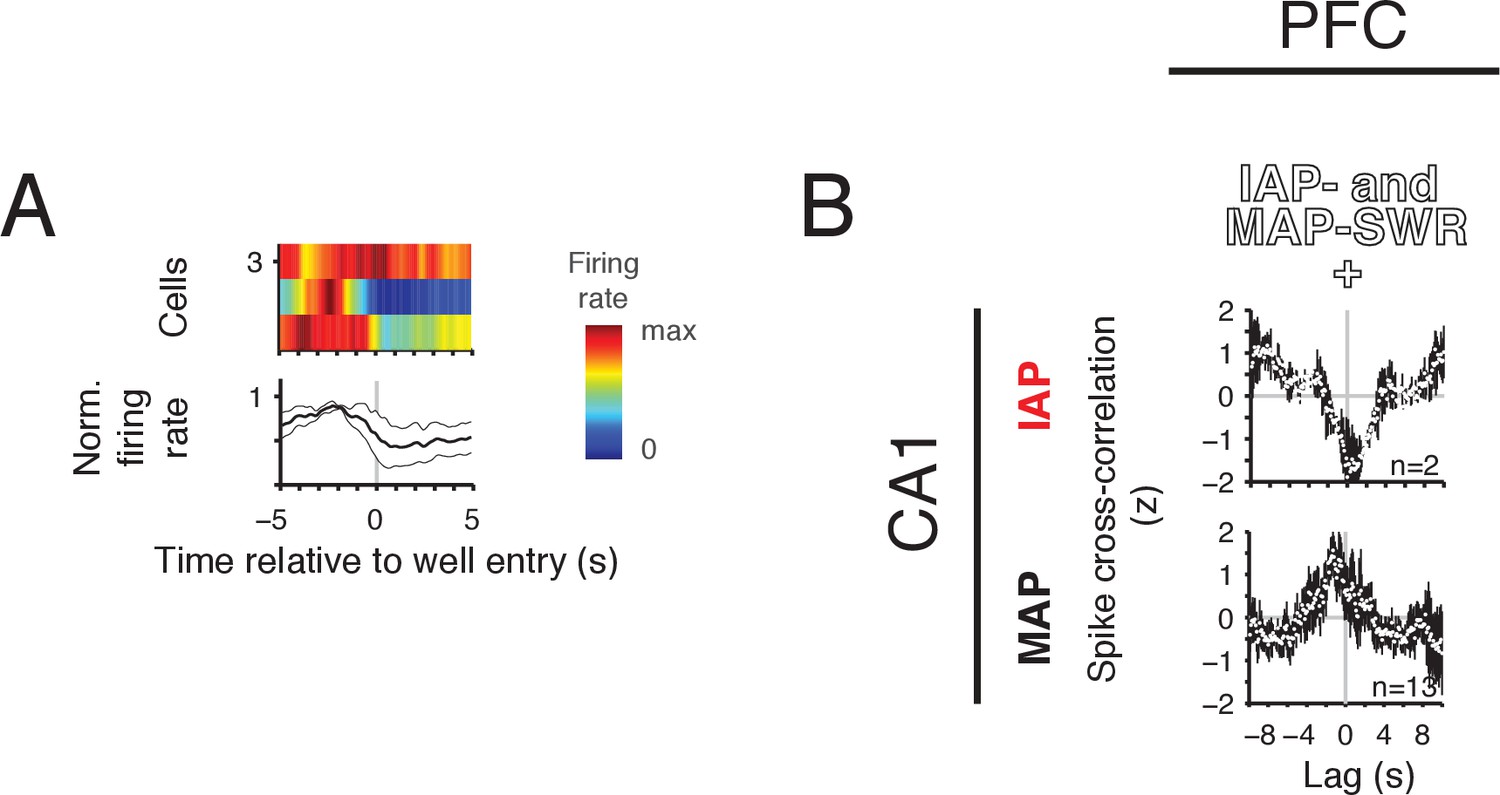
(A) Mean firing rate for PFC IAP- and MAP-SWR+ cells aligned to well entry. Top row: firing rate of each cell is normalized to maximum firing rate in the −5 s to 5 s time window. Bottom row: mean normalized firing rate (±SEM). (B) Normalized population spike cross-correlation (mean ±SEM, 100 ms bins). Top row: PFC-CA1 IAP pairs. Bottom row: PFC-CA1 MAP cell pairs. Number of cell pairs indicated.
Figure 6—figure supplement 2
Spatial and temporal proximity control for PFC activity.
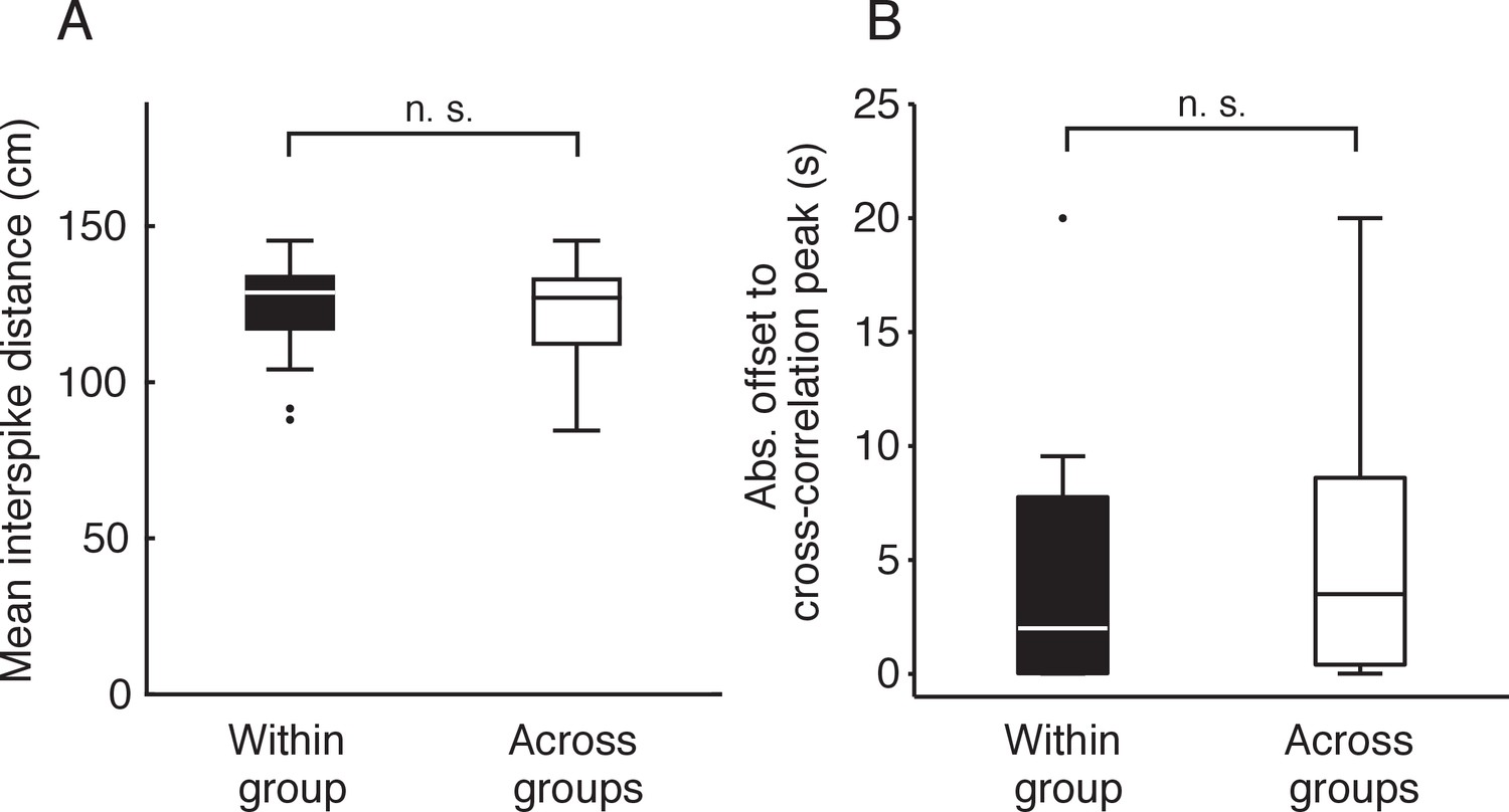
(A) Boxplot of mean inter-spike distance between cell pairs. (B) Boxplot of absolute offset to cross-correlation peak within a 20 s window for each cell pair. Within group refers to: IAP SWR+-IAP SWR+, MAP SWR+-MAP SWR+ or IAP/MAP SWR--IAP/MAP SWR- PFC cell pairs (n = 39). Across groups refers to: IAP SWR+-MAP SWR+, IAP SWR+- IAP/MAP SWR- or MAP SWR--IAP/MAP SWR- PFC cell pairs (n = 169). Wilcoxon rank-sum test: n.s. not significant.
Figure 7
A Hebbian mechanism for discretizing continuous representations of experience.
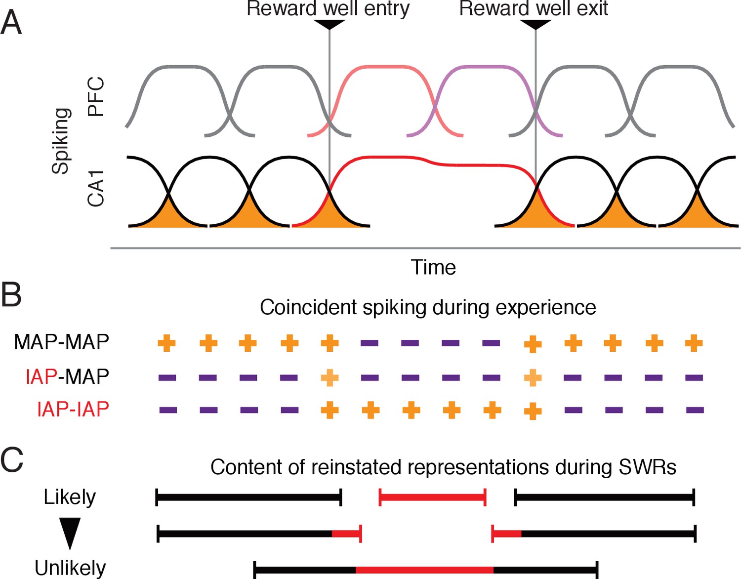
(A) Schematic of PFC and CA1 activity around reward well entry and exit. The activity of each cell over time is shown by a curve. The overlap in activity between CA1 cells is shaded orange. CA1 MAPs shown in black. CA1 IAPs shown in red. Corresponding PFC activity follows color scheme in Figure 5. (B) Schematic indicating contribution of spiking coactivity at different points in time to the strengthening of associations for MAPs and IAP pairs. Orange plus symbol indicates associations between cell pairs. The lighter shade of orange for IAP-MAP pairs indicates weaker association compared with other cell pairs. Purple minus symbol indicates weakening of associations. (C) Expected representations reactivated during SWRs based on associations in (B). Each line represents one type of reinstated representation. Black indicates movement-associated representations and red indicates immobility-associated representations.
Download links
A two-part list of links to download the article, or parts of the article, in various formats.
Downloads (link to download the article as PDF)
Open citations (links to open the citations from this article in various online reference manager services)
Cite this article (links to download the citations from this article in formats compatible with various reference manager tools)
Distinct hippocampal-cortical memory representations for experiences associated with movement versus immobility
eLife 6:e27621.
https://doi.org/10.7554/eLife.27621


