Automated long-term recording and analysis of neural activity in behaving animals
Figures
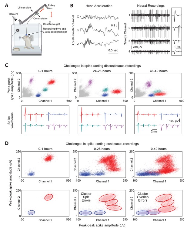
Long-term continuous neural and behavioral recordings in behaving rodents pose challenges for traditional methods of spike-sorting.
(A) Adapting our automated rodent training system (ARTS) for long-term electrophysiology. Rats engage in natural behaviors and prescribed motor tasks in their home-cages, while neural data is continuously acquired from implanted electrodes. The tethering cable connects the head-stage to a commutator mounted on a carriage that moves along a low-friction linear slide. The commutator-carriage is counterweighted to eliminate slack in the tethering cable. Behavior is continuously monitored and recorded using a camera and a 3-axis accelerometer. (B) Example of a recording segment showing high-resolution behavioral and neural data simultaneously acquired from a head-mounted 3-axis accelerometer (left) and a tetrode (right) implanted in the motor cortex, respectively. (Inset) A 2 ms zoom-in of the tetrode recording segment. (C) Drift in spike waveforms over time make it difficult to identify the same units across discontinuous recording sessions. Peak-to-peak spike amplitudes (top) and spike waveforms (bottom) for four distinct units on the same tetrode for hour-long excerpts, at 24 hr intervals, from a representative long-term continuous recording in the rat motor cortex 4 months after electrode implantation. Different units are indicated by distinct colors. We tracked units over days using a novel spike-sorting algorithm we developed to cluster continuously recorded neural data (see Figure 2). (D) Continuous extracellular recordings pose challenges for spike-sorting methods assuming stationarity in spike shapes. (Top) Peak-to-peak spike amplitudes of two continuously recorded units (same as in C) accumulated over 1 hr (left), 25 hr (middle) and 49 hr (right). (Bottom) Drift in spike waveforms can lead to inappropriate splitting (middle, right panels) of single-units and/or merging (right panel) of distinct units, even though these two units are separable in the hour-long ‘sessions’ shown in C.
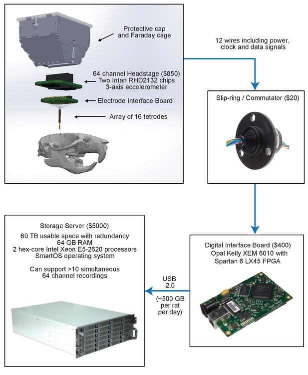
Overview of custom-built hardware for extracellular recordings in behaving rodents.
Scalable low-cost signal processing and recording hardware. Neural activity is recorded using an array of 16 tetrodes. A headstage continuously filters, amplifies, and digitizes the measured signals and sends them over to a digital interface board via a commutator. The digital interface board packages the data into USB packets and streams it to a custom-built 60 TB storage server.
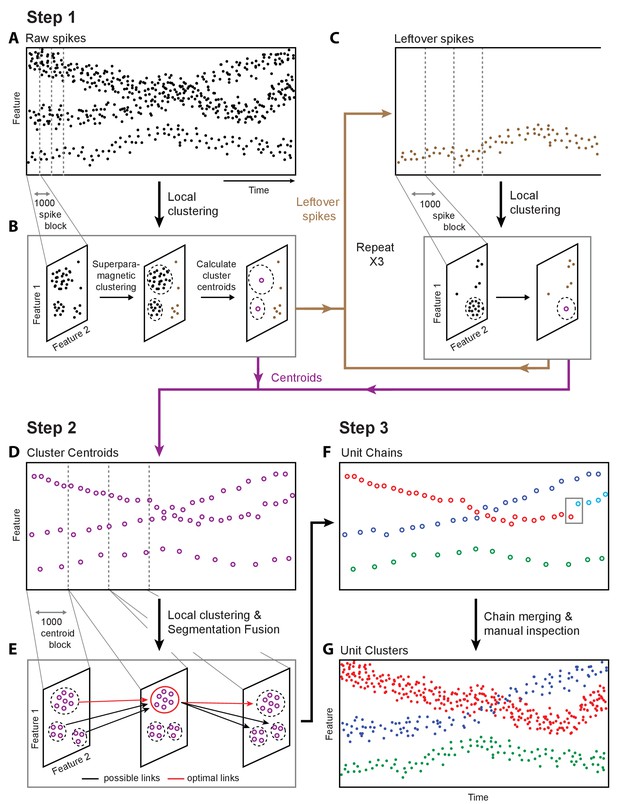
Overview of fast automated spike tracker (FAST), an unsupervised algorithm for spike-sorting continuous, long-term recordings.
(A–C) Step 1 of FAST. (A) Cartoon plot of spike waveform feature (such as amplitude) over time. Spikes are grouped into consecutive blocks of 1000 (indicated by gray dashed lines). (B) Superparamagnetic clustering is performed on each 1000 spike-block to compress and de-noise the raw spike dataset. Centroids (indicated by purple circles) of high-density clusters comprising more than 15 spikes are calculated. These correspond to units with higher firing rates. (C) Leftover spikes in low-density clusters (indicated by brown dots), corresponding to units with lower firing rates, are pooled into 1000 spike blocks and subject to the local clustering step. This process is repeated for a total of 4 iterations in order to account for spikes from units across a wide range of firing rates. Cluster centroids representing averaged spike waveforms from each round of local clustering are carried forward to Step 2 of FAST. (D–E) Step 2 of FAST. (D) Centroids from all rounds of local clustering in Step 1 are pooled into blocks of size 1000 (dashed grey lines) and local superparamagnetic clustering is performed on each block. (E) The resulting clusters are linked across time using a segmentation fusion algorithm to yield cluster-chains corresponding to single units. (F) Step 3 of FAST. In the final step, the output of the automated sorting (top) is visually inspected and similar chains merged across time to yield the final single-unit clusters (bottom).
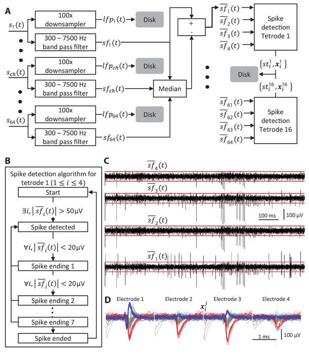
Algorithm for identifying spikes from tetrode recordings.
(A) Each input channel is split into two streams, one containing the low frequency component and one containing the high frequency one,. The median of across all channels is subtracted from each channel resulting in. Spike times and spike waveforms from each tetrode are then extracted. The LFPs and spikes extracted from the raw data are saved to disk resulting in a 5-10x ‘compression’ of the raw data. (B) Algorithm for detecting spikes. If the absolute value of the filtered signal exceeds 50 µV in any channel of a tetrode then a spike is ‘detected’. The spike is considered to have ‘ended’ if all channels remain within 20 µV for 8 consecutive samples. (C) Example of a 1 s long raw recording from a tetrode. The red lines mark the ±50 µV spike detection threshold. (D) Examples of 2.13 ms wide spike snippets (64 samples) extracted from the data in C. Snippets from all 4 electrodes detected using the state machine in B are aligned to the peak of the spike waveform and concatenated to produce the 256 sample spike waveforms.
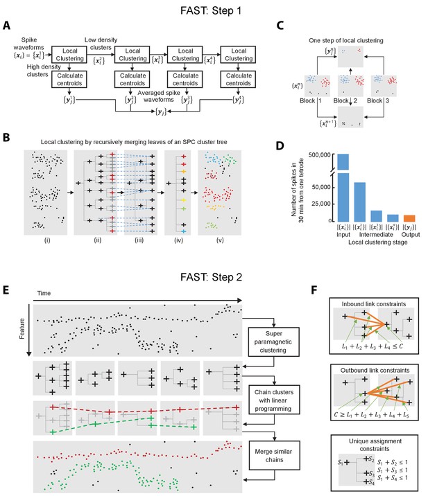
Algorithms for local clustering of spike waveforms and linking cluster trees to track units over time (Steps 1 and 2 of FAST).
(A–C) Step 1 of FAST. (A) Raw spike waveforms are locally clustered and split into low- and high-density clusters (details in panels B and C). The spikes from low-density clusters are further split into two streams in the same manner 3 more times. The centroids of high density clusters from all 4 stages are pooled together to form the output . (B) Local clustering of each 1000 spike block. Super-paramagnetic clustering generates a cluster tree (ii) from the spike waveforms (i), the leaves of which are recursively merged (iii and iv) to generate a clustering of the 1000 points (v). The dotted blue lines show which leaves of the tree in (ii) are merged to produce the tree in (iii). The nodes marked red in (ii) correspond to ‘distinct clusters’, i.e. clusters that are very different from the parent nodes. The leaves of (iii) are similarly merged to produce the tree in (iv). The colored leaves correspond to high-density clusters, i.e. clusters with more than 15 points and the black leaves correspond to low-density clusters. (C) Schematic illustrating splitting of spikes into low-density and high-density clusters. The set of input spike waveforms is split into blocks of 1000 spikes (3 blocks shown in the figure) with each block split into low (colored black) and high density clusters (colored blue and red) using the procedure shown in panel B. The spikes from the low density clusters are pooled together to form . The centroids of the high density clusters form. (D) Number of spike waveforms in a 30 min period from one tetrode in various stages of the local clustering and de-noising algorithm. (E–F) Step 2 of FAST. (E) The output of the previous steps (averaged spike waveforms as per panels A-D) is split into a blocks of 1000 averaged spikes and converted into a sequence of cluster trees (5 trees shown in the figure). A subset of all possible links between adjacent cluster trees is chosen by maximizing the total similarity between linked nodes subject to the constraints depicted in panels F. The subset of chosen nodes and links are highlighted in color. Three sets of nodes connected by links, one in red and two in green, are shown. The two green chains are merged based on waveform similarity to produce a final sorting containing two units (red and green). (F) (Top) The constraint shown ensures that none of the 4 incoming links () are chosen if the node marked is not chosen. It also ensures that if is chosen, at most one of the incoming links is chosen. (Middle) Same as above, except for outgoing links. (Bottom) These constraints ensure that if a node is chosen then none of its parents or child nodes are.
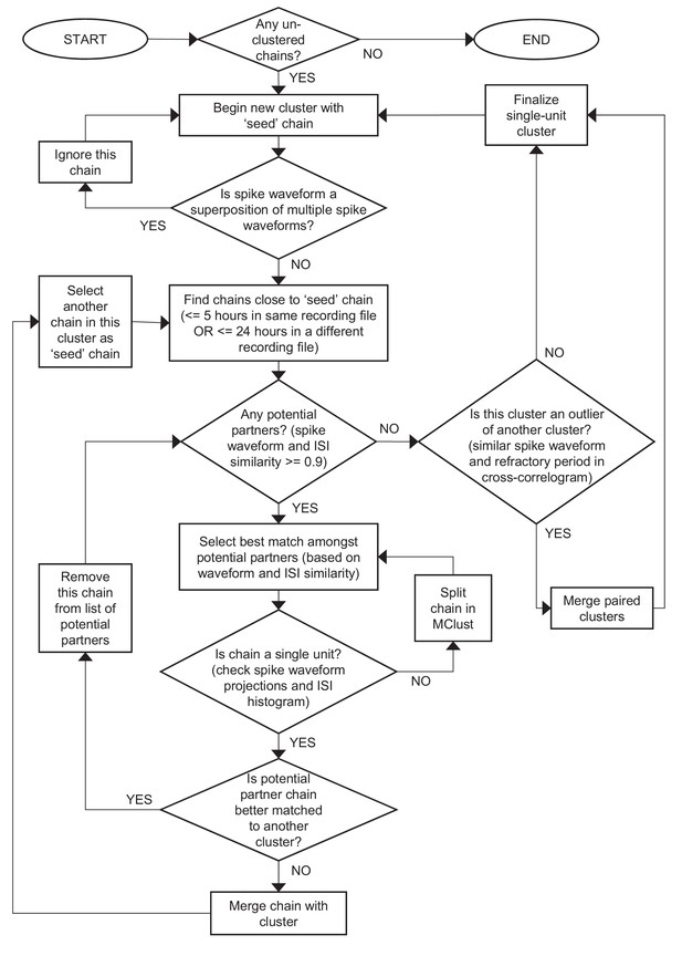
Recommended workflow for manual verification step of FAST.
See Materials and methods for more details.
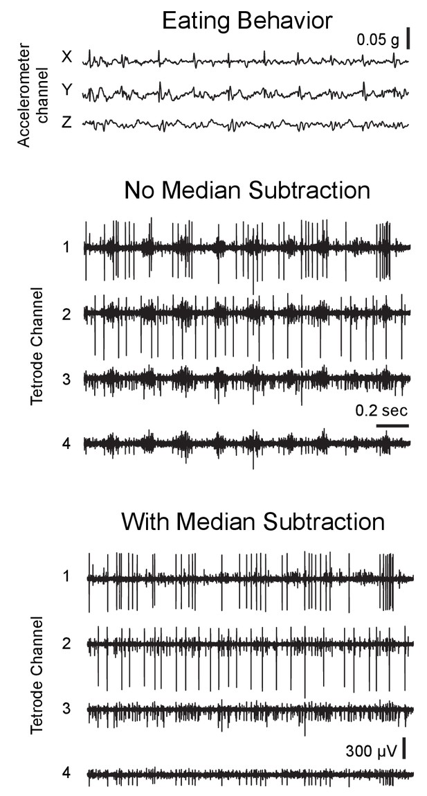
Effect of median subtraction on recording noise in behaving rats.
2 s segment of an example 3-axis accelerometer trace (top) and high-pass filtered tetrode recording from the motor cortex (middle) during eating behavior. Note the presence of correlated noise on all 4 electrode channels, presumably arising from activation of muscles responsible for chewing. (Bottom) Subtracting the median activity of all channels (as described in Figure 2—figure supplement 1) from individual electrode channels largely eliminates common-mode noise.
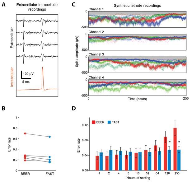
Validation of spike-sorting performance of FAST using ground-truth datasets.
(A) Example traces of simultaneous extracellular tetrode (black) and intracellular electrode (red) recordings from the anesthetized rat hippocampus (Harris et al., 2000; Henze et al., 2009). The intracellular trace can be used to identify ground-truth spike times of a single unit recorded on the tetrode. (B) Spike-sorting error rate of FAST on the paired extracellular-intracellular recording datasets (n = 5) from (Henze et al., 2009), in comparison to the best ellipsoidal error rate (BEER), a measure of the optimal performance of standard spike-sorting algorithms (see Materials and methods, Harris et al., 2000). The error rate was calculated by dividing the number of misclassified spikes (sum of false positives and false negatives) by the number of ground-truth spikes for each unit. (C) A representative synthetic tetrode recording dataset in which we model realistic fluctuations in spike amplitudes over 256 hr (see Materials and methods). The four plots show simulated spike amplitudes on the four channels of a tetrode. Colored dots indicate spikes from eight distinct units while gray dots represent multi-unit background activity. For visual clarity, we have plotted the amplitude of every 100th spike in the dataset. (D) Spike-sorting error rates of FAST (blue bars) applied to the synthetic tetrode datasets (n = 48 units from six tetrodes), in comparison to the BEER measure (red bars) over different durations of the simulated recordings. Error-bars represent standard error of the mean. * indicates p<0.05 after applying the Šidák correction for multiple comparisons.
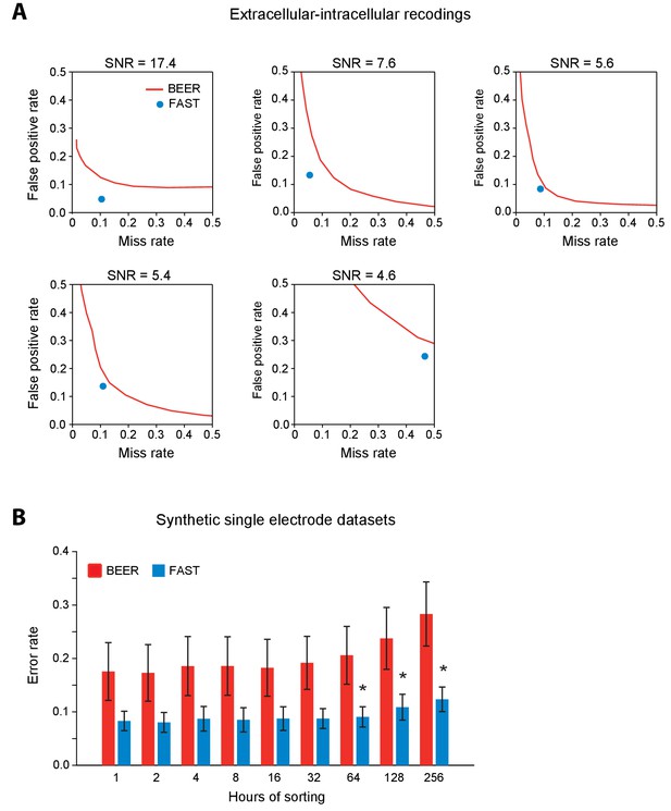
Validation of spike-sorting performance of FAST using ground-truth extracellular-intracellular recordings and synthetic single electrode datasets.
(A) Comparison of spike-sorting performance of FAST (blue dots) and BEER (best ellipsoidal error rate, red lines) on 5 different units from the extracellular-intracellular recording datasets of (Henze et al., 2009). Each plot shows the false positive versus miss (false negative) rate in clustering spikes of individual units in comparison to ground-truth. For BEER, we varied the relative misclassification cost of false-positive and miss errors in order to obtain a performance curve. SNR refers to the average signal-to-noise ratio of unit spikes in each recording. (B) Spike-sorting error rate of FAST (blue bars) applied to synthetic single electrode recordings with simulated amplitude drifts (n = 16 units from eight electrodes), in comparison to the BEER measure (red bars) over different durations of the simulated recordings ranging from 1 to the full 256 hr. Error-bars represent standard error of the mean. * indicates p<0.05 after applying the Šidák correction for multiple comparisons.
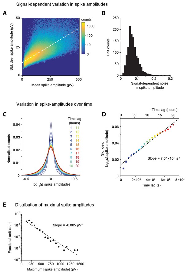
Analyzing long-term recordings in the DLS and MC to characterize variation in unit spike amplitude.
(A) Density plot of standard deviation of spike-amplitude versus mean spike amplitude computed in 1 hr blocks for all units in our DLS and MC datasets. Color scale indicates log counts. The slope of the white, dashed line of best fit represents the average signal-dependent variation in spike amplitude for the dataset (slope = 0.06). (B) Histogram of signal-dependent variation in spike amplitudes computed, as shown in A, separately for each unit in our dataset. (C) Each trace is a histogram of the difference in spike amplitudes over time-lags of 1 through 20 hr, colored as per legend, for all units in the dataset. The x-axis is plotted on a log-scale. (D) Standard deviation of histograms of log spike-amplitude differences over different time-lags from 1 to 20 hr, as shown in C. Dashed line indicates line of best fit. (E) Distribution of maximum spike amplitudes for all units in our dataset that we had recorded for at least 50 hr. The y-axis represents fractional unit counts on a log-scale. Dashed line indicates line of best fit whose slope characterizes the exponential fall-off in the fraction of units with increasing large spike amplitudes.
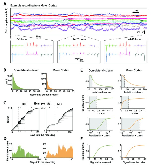
Single units isolated and tracked from continuous months-long recordings made in dorsolateral striatum (DLS) and motor cortex (MC) of behaving rats.
(A) The results of applying FAST to a representative continuous tetrode recording in the rodent motor cortex spanning 45 hr. Each point represents spike amplitudes on channel 2 of a tetrode, with different colors representing distinct units. For visual clarity we have plotted the amplitude of de-noised spike centroids (see Figure 2), not raw spike amplitudes. Insets (bottom) show average spike waveforms of six example units on the four channels of the tetrode at 0, 24 and 44 hr into the recording. (B) Holding times for all units recorded in the DLS (left, green) and MC (right, orange), sorted by duration. (C) Temporal profile of units recorded in DLS (left) and MC (right) from two example rats over a period of ~3 months. Unit recording times are indicated by black bars, and are sorted by when they were first identified in the recording. Black triangles and dotted lines indicate times at which the electrode array was intentionally advanced into the brain by turning the micro-drive. Open triangles indicate times at which the population of recorded units changed spontaneously. Number of simultaneously recorded units in the DLS (left, green) and MC (right, orange) as a function of time in the two example recordings. (D) Number of simultaneously recorded units in the DLS (left, green) and MC (right, orange) as a function of time in the example recordings shown in C. (E) Cumulative distributions of average cluster isolation quality for all units recorded in DLS (left, green) and MC (right, orange). Cluster quality was measured by the isolation distance (top), L-ratio (middle), and fraction of inter-spike intervals under 2 ms (bottom). Dotted lines mark the quality thresholds for each of these measures. Shaded regions denote acceptable values. (F) Cumulative distributions of average signal-to-noise ratios for all units recorded in DLS (left, green) and MC (right, orange).
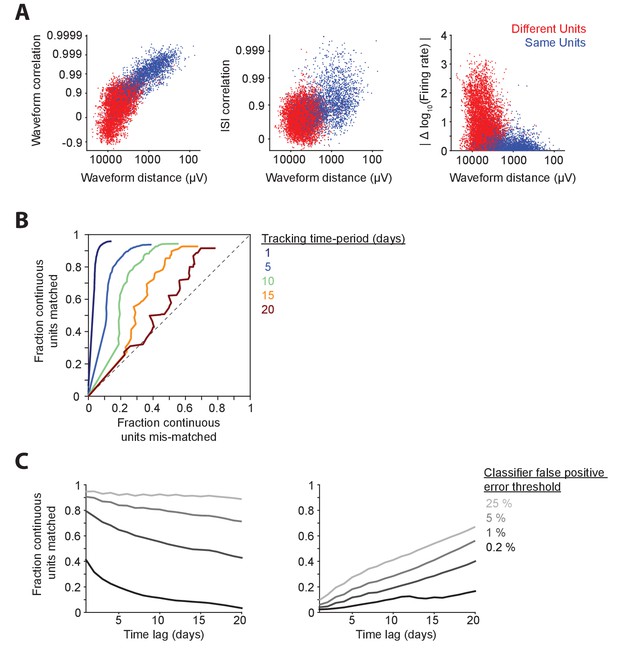
Benchmarking the performance of discontinuous unit-tracking methods using continuous long-term datasets sorted by FAST.
(A) Discontinuous tracking of units across daily recording sessions is error-prone. Similarity metrics between units isolated on consecutive days in hour-long recording sessions (data from an example DLS recording). Three out of six possible combinations of similarity features are presented here – spike waveform correlation (left), inter-spike interval histogram (ISI) correlation (middle) and absolute log firing rate difference (right) versus spike waveform Euclidean distance. Each dot represents the similarity between pairs of units recorded on the same tetrode and classified as the ‘same’ (blue dot) or ‘different’ (red dot) by our FAST algorithm. (B) Receiver-operator characteristic (ROC) curves for discontinuous tracking of units over time-periods of 1, 5, 10, 5 and 20 days. Each ROC curve was generated by systematically varying the desired false-positive error rate of a ‘same’ versus ‘different’ optimal linear classifier from 0% to 100%. Line colors indicate different tracking time-periods as per the plot legend. Note that the discontinuous tracking algorithm (see Materials and methods) matches pairs of units across days in order of their similarity, with highest similarity pairs being matched first. Due to this, the fraction of units mis-matched (false positive error rate of unit tracking) does not reach 100% even when the desired false-positive error rate of the ‘same’ v/s ‘different’ classifier is set to 100%. (C) (Left) Percentage of ‘same’ unit pairs identified by the FAST method that were successfully matched by discontinuous tracking at 1 day intervals, over time-periods ranging from 1 to 20 days. (Right) Percentage of discontinuously matched unit pairs that are classified as ‘different’ by FAST for time-periods ranging from 1 to 20 days. Graded colors correspond to different false positive rate thresholds of the ‘same’ versus ‘different’ optimal linear classifier (see Materials and methods) ranging from 0.2% (light gray) to 25% (black).
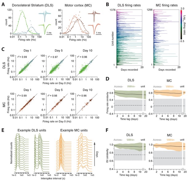
Long-term stability of single unit activity.
(A) Histograms of average firing rates for units recorded in DLS (left) and MC (right). Putative cell-types, medium spiny neurons (MSN, blue) and fast-spiking interneurons (FSI, green) in DLS, and regular spiking (RS, brown) and fast spiking (FS, red) neurons in the MC, were classified based on spike shape and firing rate (Materials and methods). The continuous traces are log-normal fits to the firing rate distributions of each putative cell-type. Insets show average peak-normalized waveform shapes for MSNs (left-bottom) and FSIs (left-top), and RS (right-bottom) and FS (right-top) neurons. Shading represents the standard deviation of the spike waveforms. (B) Firing rates of DLS (left) and MC (right) units over 20 days of recording. The color scale indicates firing rate on a log-scale, calculated in one-hour blocks. Units have been sorted by average firing rate. (C) Scatter plots of unit firing rates over time-lags of 1 (left), 5 (middle) and 10 (right) days for DLS (top) and MC (bottom). The dashed lines indicate equality. Every dot is a comparison of a unit’s firing from a baseline day to 1, 5 or 10 days later. The color of the dot indicates putative cell-type as per (A). Each unit may contribute multiple data points, depending on the length of the recording. Day 1: n = 4398 comparisons for striatum and n = 1458 for cortex; Day 5: n = 2471 comparisons for striatum and n = 615 for cortex; Day 10: n = 1347 comparisons for striatum and n = 268 for cortex. (D) Stability of unit firing rates over time. The firing rate similarity (see Materials and methods) was measured across time-lags of 1 to 20 days for the same unit (within-unit, solid lines), or between simultaneously recorded units (across-unit, dashed lines) in DLS (left) and MC (right). Colored shaded regions indicate the standard deviation of within-unit firing rate similarity, over all units. Grey shaded regions indicate standard deviation of across-unit firing rate similarity, over all time-bins. (E) Inter-spike interval (ISI) histograms for example units in DLS (left, green) and MC (right, orange) over two weeks of continuous recordings. Each line represents the normalized ISI histogram measured on a particular day. (F) Stability of unit ISI distributions over time. Correlations between ISI distributions were measured across time-lags of 1 to 20 days for the same unit (within-unit, solid lines), or between simultaneously recorded units (across-unit, dashed lines) in DLS (left) and MC (right). Colored shaded regions indicate the standard deviation of within-unit ISI similarity, over all units. Grey shaded regions indicate standard deviation of across-unit ISI similarity, over all time-bins.
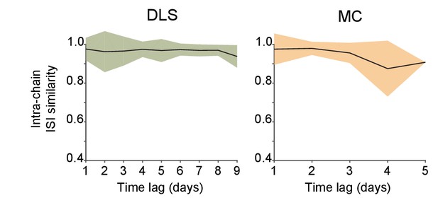
Stability over time of ISI distributions computed from spike chains that were automatically identified by FAST.
Stability of chain-derived ISI distributions over time. Correlations between ISI distributions were measured across time-lags of 1 to 9 days for the same chain in DLS (left) and across time-lags of 1 to 5 days for chains in MC (right). Colored shaded regions indicate the standard deviation of within-chain ISI similarity, over all chains.
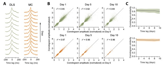
Stability of network dynamics.
(A) Correlograms for example unit pairs from DLS (left) and MC (right) over 10+ days. Each line represents the normalized correlogram measured on a particular day. (B) Scatter plots comparing the correlogram amplitude (normalized) of a unit pair on a baseline day to the same pair’s peak correlation 1, 5 or 10 days later, for DLS (top) and MC (bottom). The black line indicates equality. Values > 1 (or <1) correspond to positive (or negative) correlations (see Materials and methods). Day 1: n = 48472 comparisons for DLS and n = 12148 for MC. Day 5: n = 19230 comparisons for DLS and n = 2881 for MC. Day 10: n = 7447 comparisons for DLS and n = 772 for MC. All unit pairs whose correlograms had at least 5000 spikes over a day’s period were included. (C) Stability of correlations over time. The correlogram similarity (see Materials and methods) was measured across time-lags of 1 to 10 days for pairs of units (solid lines) in DLS (top) and MC (bottom). Colored shaded regions indicate the standard deviation of the correlogram similarity between all pairs that had significant correlograms on at least one recording day (Materials and methods).
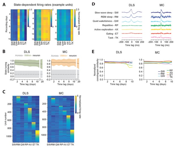
Stability of behavioral state-dependent activity patterns.
(A) Stability of average firing rates in different behavioral states (i.e. the unit’s ‘state-tuning’) across several days for example units recorded in the DLS (left) and MC (middle and right). The color-scale corresponds to the firing rate of a unit normalized by its average firing rate. The state abbreviations correspond to slow-wave sleep (SW), REM sleep (RM), quiet wakefulness (QW), repetitive (RP), active exploration (AX), eating (ET) and task execution (TK). (B) Stability of units’ state-tuning over time. Correlations between the state-tuning profiles (as in ‘A’) were measured across time-lags of 1 to 20 days for the same unit (within-unit, solid lines), or between simultaneously recorded units (across-unit, dashed lines) in MC (left) and DLS (right). Colored shaded regions indicate the standard deviation of within-unit state-tuning similarity, over all units. Grey shaded regions indicate standard deviation of across-unit state-tuning similarity, over all time-bins. (C) Diversity in state-tuning across all units recorded in the DLS (left) and MC (right). Units are sorted by the peak behavioral state in their state-tuning curves. (D) Cross-correlograms computed for example pairs of units in the DLS (left) and MC (right) in different behavioral states. Line colors represent behavioral state. (E) Stability of cross-correlograms measured within specific behavioral states. The correlation similarity (see Materials and methods) was measured across time-lags of 1 to 10 days (solid lines) in DLS (left) and MC (right). Line colors represent correlation similarity for different behavioral states, as per the plot legend.
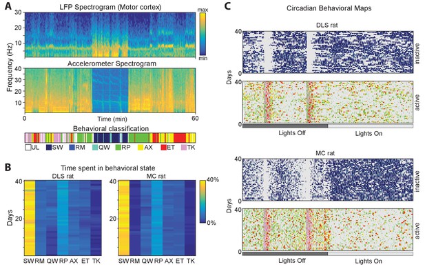
Automated classification of behavioral states.
(A) (Top) Spectrograms of the accelerometer signal (top) and the LFP (middle) for an hour-long window of recording from the motor cortex. Below is the color-coded output of our automated classification algorithm. UL-unlabeled; SW-Slow wave sleep; RM-REM sleep; QW- quiet wakefulness, RP-repetitive behavior, AX-active exploration, ET-eating, TK-task. (B) Ethograms showing the proportion of time spent in each of the behavioral states over 40 consecutive days for two example rats. The ethograms do not include absence seizure-like states or unlabeled states (Materials and methods). (C) Circadian profiles of behavioral states over 40 days of recording for active and inactive states for the two rats in B. Behavioral states are color-coded as in A, with gray representing inactive (or active) and unlabeled states.
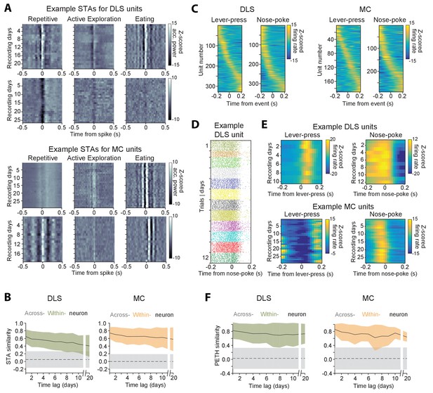
Stability of behavioral representations.
(A) Spike-triggered average (STA) accelerometer power calculated daily in three different behavioral states – repetitive behavior (left), active exploration (middle) and eating (right). Shown are four example units recorded from DLS (top two rows) and MC (bottom two rows). (B) Stability of STAs over time. Correlations between STAs were measured across time-lags of 1 to 20 days for the same unit (within-unit, solid lines), or between simultaneously recorded units (across-unit, dashed lines) in DLS (left) and MC (right). Colored shaded regions indicate the standard deviation of within-unit STA similarity (averaged over the three behavioral states in ‘A’), over all units. Grey shaded regions indicate standard deviation of across-unit STA similarity, over all time-bins. (C) Peri-event time histograms (PETHs) of DLS (left) and MC (right) unit activity, aligned to the timing of a lever-press or nose-poke during the execution of a skilled motor task. Plotted are the PETHs of units that had significant modulations in their firing rate in a time-window ±200 ms around the time of the behavioral event (Materials and methods). The color scale indicates Z-scored firing rate. Units are sorted based on the times of peaks in their PETHs. (D) Spike raster of an example DLS unit over 12 days, aligned to the time of a nose-poke event. Each dot represents a spike-time on a particular trial. The color of the dot indicates day of recording. (E) PETHs computed over several days for example DLS (top) and MC (bottom) units to lever-press (left) and nose-poke (right) events in our task. (F) Stability of task PETHs over time. Correlations between PETHs were measured across time-lags of 1 to 20 days for the same unit (within-unit, solid lines), or between simultaneously recorded units (across-unit, dashed lines) in DLS (left) and MC (right). Colored shaded regions indicate the standard deviation of within-unit PETH similarity (averages across lever-press and nose-poke events), over all units. Grey shaded regions indicate standard deviation of across-unit PETH similarity (averaged across lever-press and nose-poke events), over all time-bins.
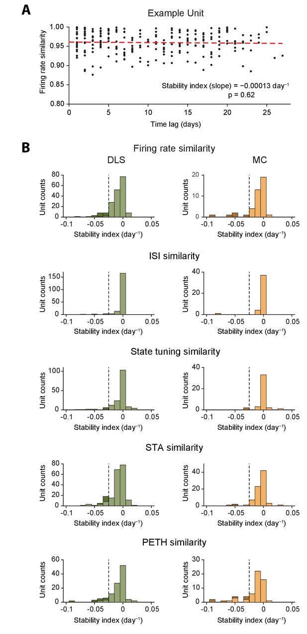
Measurements of long-term stability of neural dynamics and motor representations for individual units.
(A) Measuring firing rate stability for an example unit recorded in the DLS. The plot shows firing rate similarity (see Figure 5 and Materials and methods) plotted against time-lag in days. Each dot represents a different comparison. The stability of firing rate similarity (the stability index) is measured by fitting a regression line (indicated by red dashes) to the data and calculating its slope and p-value. (B) Histograms of stability indices for different metrics of neural dynamics for all units recorded in the DLS (left) and MC (right), computed as shown in A. Shaded bars indicate counts of units with significantly low stability indices (stability index < -0.025 day−1 and p<0.05 after applying the Šidák correction for multiple comparisons). See Table 2 for quantification of the number of units with significantly low stability indices. The vertical dashed line indicates the stability threshold (0.025 day−1).
Tables
Proportion of units that have stable neural dynamics and motor representations in the striatum and motor cortex.
https://doi.org/10.7554/eLife.27702.021| Activity metric | Dorsolateral striatum | Motor cortex | ||
|---|---|---|---|---|
| % stable | n | % stable | n | |
| Firing rate | 90.3 | 186 | 88.1 | 42 |
| ISI histogram | 97.9 | 187 | 97.6 | 42 |
| State tuning | 93.9 | 163 | 92.7 | 41 |
| STA | 93.6 | 202 | 95.0 | 80 |
| PETH | 89.4 | 113 | 89.5 | 57 |
List of parameters for the fully automated steps of FAST and their recommended values.
https://doi.org/10.7554/eLife.27702.022| Step | Parameter | Details | Recommended value |
|---|---|---|---|
| Snippeting | block size | Length of data segment to filter and snippet per block | 15 s |
| Snippeting | end padding | To account for edge effects in filtering | 100 ms |
| Snippeting | waveform samples pre and post | Samples per spike snippet to record before and after peak (not including peak sample) | 31 and 32 samples (total 64 samples @ 30 kHz sampling) |
| Snippeting | spike detection threshold | Threshold voltage to detect spikes | 7 × median absolute deviation of recording |
| Snippeting | spike return threshold | Threshold voltage below which the spike detection process is reset | 3 × median absolute deviation of recording |
| Snippeting | spike return number of samples | Number of samples the recorded voltage must stay under the spike return threshold to reset the spike detection process | 8 samples (0.27 ms @ 30 kHZ sampling rate) |
| Clustering: Step 1 | spikes per block | Number of spikes per block for local clustering | 1000 spikes |
| Clustering: Step 1 | minimum and maximum SPC temps | Range of temperatures for super-paramagnetic clustering (SPC) | 0, 15 |
| Clustering: Step 1 | Threshold for recursive merging of SPC tree (‘a’) | Threshold distance between leaf node and its parent node in the SPC tree below which the leaf node is merged with its parent. | 20 µV |
| Clustering: Step 1 | Minimum cluster size | Min. number of spikes in cluster to compute cluster centroid | 15 spikes |
| Clustering: Step 1 | Number of rounds of local clustering | Rounds of iterative multi-scale clustering | 4 |
| Clustering: Step 2 | Spike centroids per block | Number of spike cluster centroids per block for generating SPC tree prior to segmentation fusion | 1000 centroids |
| Clustering: Step 2 | Cluster trees per block | Number of cluster trees per block for segmentation fusion | 10 cluster trees |
| Clustering: Step 2 | Segmentation fusion block overlap | Number of cluster trees overlap between blocks for segmentation fusion | 5 cluster trees |
| Clustering: Step 2 | ‘s’, ‘k’ | Parameters for sigmoid scaling of link weights to be between 0 and 1 in segmentation fusion | s = 0.005, k = 0.03 |
| Clustering: Step 2 | Link similarity threshold | Similarity threshold for link weights between cluster trees in segmentation fusion | 0.02 (range 0–1) |
| Clustering: Step 2 | Link similarity threshold for straggler nodes | Similarity threshold for joining leftover nodes to an existing chain in segmentation fusion | 0.02 (range 0–1) |
Additional files
-
Transparent reporting form
- https://doi.org/10.7554/eLife.27702.023


