Affective bias as a rational response to the statistics of rewards and punishments
Figures
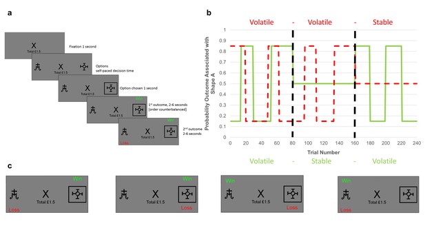
Task structure.
(A) Timeline of one trial from the learning task used in this study. Participants were presented with two shapes (referred to as shape ‘A’ and ‘B’) and had to choose one. On each trial, one of the two shapes was be associated with a ‘win’ outcome (resulting in a win of 15 p) and one with a ‘loss’ outcome (resulting in a loss of 15 p). The two outcomes were independent, that is knowledge of the location of the win provided no information about the location of the loss (see description of panel C below). Using trial and error participants had to learn where the win and loss were likely to be found and use this information to guide their choice in order to maximise their monetary earnings. (B) Overall task structure. The task consisted of 3 blocks of 80 trials each (i.e. vertical, dashed, dark lines separate the blocks). The y-axis represents the probability, p, that an outcome (win in solid green or loss in dashed red) will be found under shape ‘A’ (the probability that it is under shape ‘B’ is 1-p). The blocks differed in how volatile (changeable) the outcome probabilities were. Within the first block both win and loss outcomes were volatile, in the second two blocks one outcome was volatile and the other stable (here wins are stable in the second block and losses stable in the third block). The volatility of the outcome influences how informative that outcome is. Consider the second block in which the losses are volatile and the wins stable. Here, regardless of whether the win is found under shape ‘A’ or shape ‘B’ on a trial, it will have the same chance of being under each shape in the following trials, so the position of a win in this block provides little information about the outcome of future trials. In contrast, if a loss is found under shape ‘A’, it is more likely to occur under this shape in future trials than if it is found under shape ‘B’. Thus, for the second block losses provide more information than wins and participants are expected to learn more from them. (C) The four potential outcomes from a trial. Win and loss outcomes were independent, and so participants had to separately estimate where the win and where the loss would be on each trial in order to complete the task. This manipulation made it possible to independently manipulate the volatility of the two outcomes.
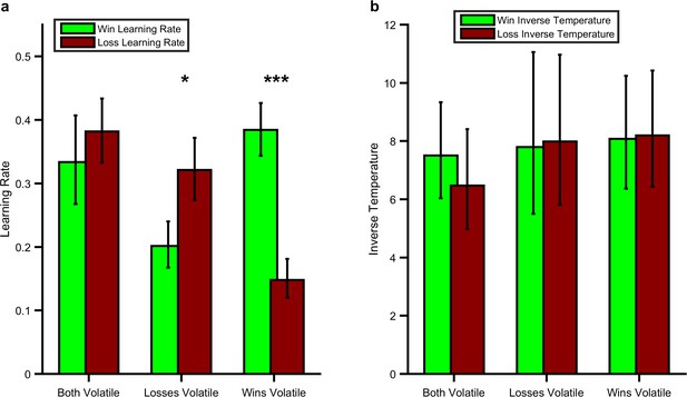
Effect of the Volatility Manipulation on Participant Behaviour.
(A) Mean (SEM) learning rates for each block of the learning task. As can be seen the win learning rates (light green bars) and loss learning rate (dark red bars) varied independently as a function of the volatility of the relevant outcome F(1,28) =27.97, p<0.001, with a higher learning rate being used when the outcome was volatile than stable (*p<0.05, ***p<0.001 for pairwise comparisons). (B) No effect of volatility was observed for the inverse temperature parameters (F(1,28) =0.01, p=0.92). Source data available as Figure 2—source data 1. See Figure 2—figure supplement 1 for an analysis of this behavioural effect which does not rely on formal modelling and Figure 2—figure supplement 2 for an additional task which examines the behavioural effect of expected uncertainty.
-
Figure 2—source data 1
Fitted model parameters, questionnaire measures and mean pupil response to volatility for all participants.
- https://doi.org/10.7554/eLife.27879.007
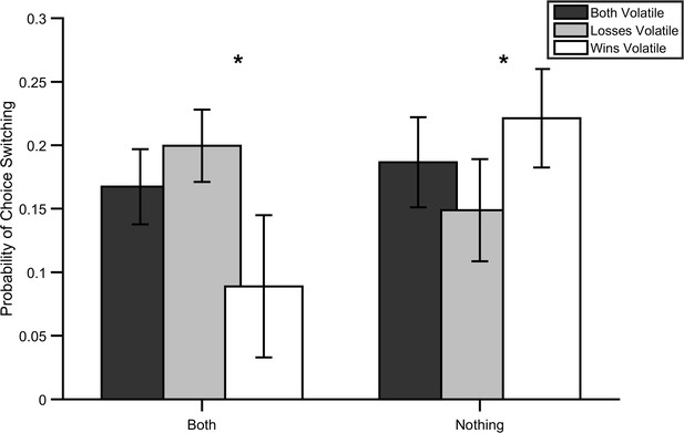
Analysis of switching behaviour in the learning task.
The learning task includes both positive and negative outcomes which are independent of each other. As a result the task contains trials in which both positive and negative outcome encourage the same behaviour in future trials (e.g. when the win is associated with shape A and the loss with shape B, both outcomes encourage selection of shape A in the following trial) as well as trials in which the positive and negative outcomes act in opposition (e.g. when both outcomes are associated with shape A, then the win outcome encourages selection of shape A in the next trial and the loss outcome encourages selection of shape B). This second type of trial provides a simple and sensitive means of assessing how the volatility manipulations alters the impact of win and loss outcomes on choice behaviour in the task blocks. Specifically an increased influence of win outcomes (e.g. when wins are volatile) should lead to: (a) A decreased tendency to change (shift) choice when both win and loss outcomes are associated with the chosen shape in the current trial and (b) An increased tendency to change (shift) choice when both win and loss outcomes are associated with the unchosen shape in the current trial. This analysis does not depend on any formal model and thus can be used to complement the model based analysis reported in the main paper. We calculated the proportion of shift trials separately for trials in which both outcomes were associated with the chosen (‘both’) or unchosen (‘nothing’) shape for each of the three blocks (dark columns = both informative; grey columns = losses informative; white columns = wins informative). Consistent with the model based analysis, there was a significant interaction between trial type and block (F(1,28)=10.52, p=0.003). Participants switched significantly less frequently when both outcomes were associated with the chosen option in the win relative to loss informative blocks (F(1,28)=6.1, p=0.02) and switched significantly more frequently when both outcomes were associated with the unchosen option in the win relative to loss informative blocks (F(1,28)=4.69, p=0.04). This indicates that the results reported in the main paper are unlikely to be dependent on the exact form of the behavioural model used to derive the learning rate parameter. Bars represent mean (SEM) probability of switching choice in subsequent trial. *=p < 0.05 for comparison between win informative and loss informative blocks.
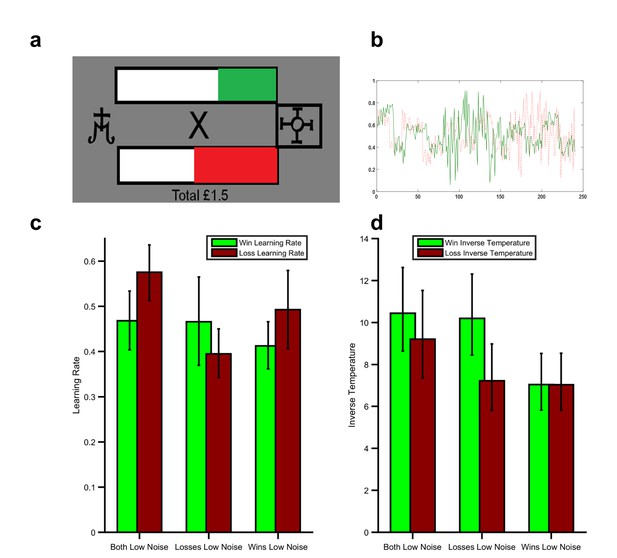
Magnitude task.
When learning, a number of different forms of uncertainty can influence behaviour. One form, which is sometimes called ‘unexpected uncertainty’ (Yu and Dayan, 2005) is caused by changes in the associations being learned (i.e. volatility) and is the main focus of this paper (see main text for a description of how volatility influences learning). A second form of uncertainty, sometimes called ‘expected uncertainty’(Yu and Dayan, 2005) arises when an association between a stimulus or action and the subsequent outcome is more or less predictive. For example, this form of uncertainty is lower if an outcome occurs on 90% of the times an action is taken and higher if the outcome occurs on 50% of the time an action is taken. Normatively, expected uncertainty should influence learning rate—a less predictive association (i.e. higher expected uncertainty) leads to more random outcomes which tell us less about the underlying association we are trying to learn, so learners should employ a lower learning rate when expected uncertainty is higher. In the learning task described in this paper both the expected and unexpected uncertainty differ between blocks. Specifically, when an outcome is stable in the task it occurs on 50% of trials, whereas when it is volatile it varies between occurring on 85/15% of trials. Thus the stable outcome is, at any one time, also less predictable (i.e. noisier) than the volatile outcome. This task schedule was used as a probability of 50% for the stable outcome improves the ability of the task to accurately estimate learning rates (it allows more frequent switches in choice). Further both forms of uncertainty would be expected to reduce learning rate in the stable blocks and increase it in the volatile block of the task. However, this aspect of the task raises the possibility that the observed effects on behaviour described in the main paper may arise secondary to differences in expected uncertainty (noise) rather than the unexpected uncertainty (volatility) manipulation. In order to test this possibility we developed a similar learning task in which volatility was kept constant and expected uncertainty was varied. In this magnitude task (panel a), participants again had to choose between two shapes in order to win as much money as possible. On each trial 100 ‘win points’ (bar on top of fixation cross with green fill) and 100 ‘loss points’ (bar under fixation cross with red fill) were divided between the two shapes and participants received money proportional to the number of win points – loss points of their chosen option. Thus, a win and loss outcome occurred on every trial of this task, but the magnitude of these outcomes varied. During the task, participants had to learn the expected magnitude of wins and losses for the shapes rather than the probability of their occurrence. This design allowed us to present participants with schedules in which the volatility (i.e. unexpected uncertainty) of win and loss magnitudes was constant (three change points occurred per block) but the noise (expected uncertainty) varied (Panel b; the standard deviation of the magnitudes was 17.5 for the high noise outcomes and 5 for the low noise outcomes). Otherwise the task was structurally identical to the task reported in the paper with 240 trials split into three blocks. We recruited a separate cohort of 30 healthy participants who completed this task and then estimated their learning rate using a model which was structurally identical (i.e. two learning rates and two inverse temperature parameters) to that used in the main paper (Model 1). As can be seen (Panel c), there was no effect of expected uncertainty on participant learning rate (block information x parameter valence; F(1,28)=1.97, p=0.17) during this task. This suggests that the learning rate effect reported in the paper cannot be accounted for by differences in expected uncertainty and therefore is likely to have arisen due to the unexpected uncertainty (volatility) manipulation. Inverse decision temperature did differ between block (Panel d; F(1,28)=5.56, p=0.026). As can be seen there was a significantly higher win inverse temperature during the block in which the losses had lower noise (F(1,28)=9.26,p=0.005) and when compared to the win inverse temperature when wins had lower noise (F(1,28)=5.35,p=0.028), but no equivalent effect for loss inverse temperature. These results indicate that, if anything, participants were more influenced by noisy outcomes. Interestingly a previous study (Nassar et al., 2012) described a learning tasks in which a normative effect of outcome noise was seen (i.e. a higher learning rate was used by participants when the outcome had lower noise). The task used by Nassar and colleagues differed in a number of respects to that used here (only rewarding outcomes were received and participants had to estimate a number on a continuous scale, based on previous outcomes rather than make a binary choice) which may explain why an effect on learning rate was not observed in the current task. Regardless of the exact reason for the lack of effect of noise in the magnitude task, it suggests that the effect described in the main paper is likely to be driven by an effect of unexpected rather than expected uncertainty.
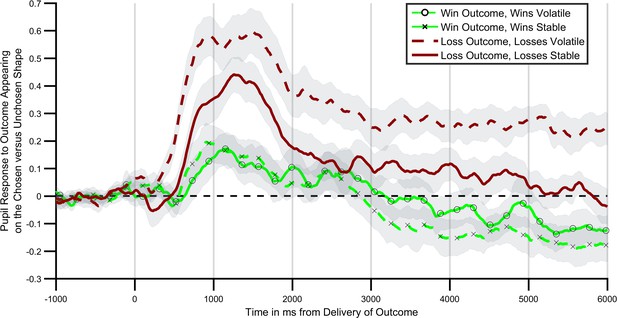
Pupil response to outcome delivery during the learning task.
Lines illustrate the mean pupil dilation to an outcome when it appears on the chosen relative to the unchosen shape, across the 6 s after outcomes were presented. Light green lines (with crosses and circles) report response to win outcomes, dark red lines report response to loss outcomes. Solid lines report blocks in which the wins were more informative (volatile), dashed lines blocks in which losses were more informative. As can be seen pupils dilated more when the relevant outcome was more informative, with this effect being particularly marked for loss outcomes. Shaded regions represent the SEM. Figure 3—figure supplement 1 plots the timecourses for trials in which outcomes were or were not obtained separately, and Figure 3—figure supplement 2 reports the results of a complimentary regression analysis of the pupil data.
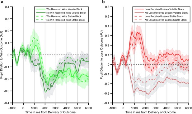
Individual time courses for trials in which wins (panel a) and losses (panel b) are either received or not received.
Lines represent the mean and shaded areas the SEM of pupil dilation over the 6 s after outcomes are presented. Figure 3 illustrates the difference in pupil dilation between trials in which an outcome was received and those in which the outcome was not received. In order to further investigate this effect the mean pupil response for trials in which the outcome was and was not received have been separately plotted. As can be seen, whereas there is relatively little difference in pupil response during the win trials, there is a large difference in dilation between trials on which a loss is received and those in which no loss is received. Further, the effect of loss volatility is seen to both increase dilation on receipt of a loss and reduce dilation when no loss is received, suggesting that the effect of the volatility manipulation is to exaggerate the effect of the outcome.
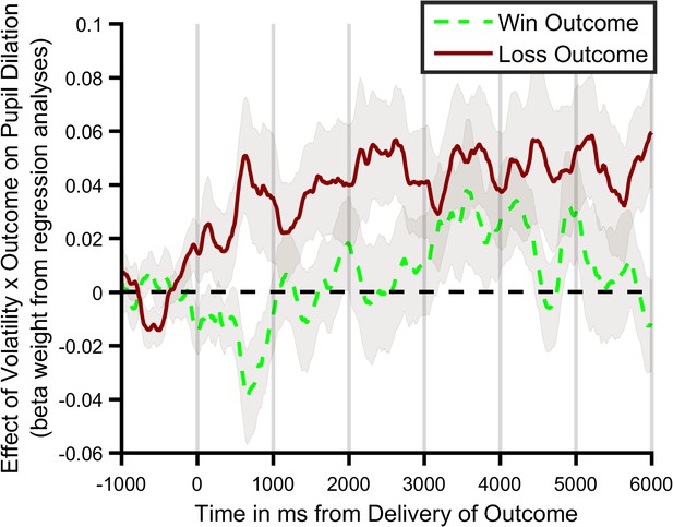
Regression analysis of pupil data.
The analysis of pupil data reported in the main text examines the effect of block information content (i.e. win volatile vs. loss volatile) and outcome receipt on the pupil response to win and loss outcomes. However a number of other factors may also influence pupil dilation such as the order in which the outcomes were presented and the surprise associated with the outcome (Browning et al., 2015). In order to ensure that these additional factors could not account for our findings we ran a regression analysis of the pupil data from the learning task. In this analysis we derived, for each participant, trialwise estimates of the outcome volatility and outcome surprise of the chosen option using the Ideal Bayesian Observer reported by Behrens et al. (Behrens et al., 2007). These estimates were entered as explanatory variables alongside variables coding for outcome order (i.e. win displayed first or second), outcome of the trial (outcome received or not) and an additional term coding for the interaction between the outcome volatility and outcome of the trial (i.e. analogous to the pupil effect reported in Figure 3). Separate regression analyses were run for each 2 ms timepoint across the outcome period, for win and loss outcomes and for each participant. This resulted in timeseries of beta weights representing the impact of each explanatory factor, for each participant and for win and loss outcomes. As can be seen, consistent with the results reported in the paper this analysis revealed a significant volatility x outcome interaction for loss outcomes (F(1,27)=6.249, p=0.019), with no effect for wins (F(1,27)=0.215, p=0.646). This result indicates that the pupil effects reported in the main paper are not the result of outcome order or surprise effects on pupil dilation. Lines illustrates mean (SEM) beta weight of the volatility x outcome regressors for win (green) and loss (red) outcomes.
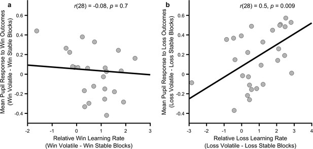
Relationship between behavioural and physiological measures.
The more an individual altered their loss learning rate between blocks, the more that individual’s pupil dilation in response to loss outcomes differed between the blocks (panel b; p=0.009), however no such relationship was observed for the win outcomes (panel a; p=0.7). Note that learning rates are transformed onto the real line using an inverse logit transform before their difference is calculated and thus the difference score may be greater than ±1. Figure 4—figure supplements 1 and 2 describe the relationship between these measures and baseline symptoms of anxiety and depression.
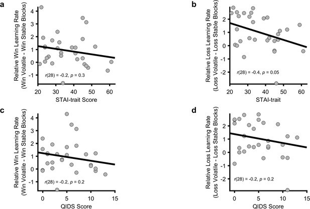
Relationship between symptom scores and behavioural adaptation to volatility.
Although participants in the current study were not selected on the basis of their symptoms of depression or anxiety, baseline questionnaires were completed allowing assessment of the relationship between symptoms and task performance. A correlation was found between trait-STAI and the change in learning rate to losses, with participants with higher scores adjusting their learning rate less than those with a lower score (Panel b; r = −0.36, p=0.048). This is the same effect reported by Browning et al., 2015. We did not observe any relationship between either questionnaire measure and change in the win learning rate or between QIDS score and change in loss learning rate (Panels a, c, d; all p>0.19).
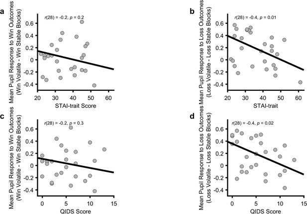
Relationship between symptom scores and pupillary adaptation to volatility.
Consistent with previous work (Browning et al., 2015) symptoms of anxiety, measured using the trait-STAI and depression, measured using the QIDS, correlated significantly negatively with differential pupil response to losses (Panels c, d; all r < −0.43, all p<0.02). That is, the higher the symptom score, the less pupil dilation differed between the loss informative and loss non-informative blocks. These measures did not correlate with pupil response to wins (Panels a, c; all p>0.19).
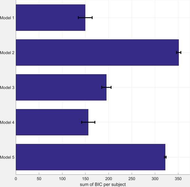
BIC Scores for Comparator Models (see table S1 for model descriptions).
Smaller BIC scores indicate a better model fit. BIC scores were calculated as the sum across all three task blocks. Bars represent mean (SEM) of the scores across participants.
Tables
Demographic details of participants
https://doi.org/10.7554/eLife.27879.003| Measure | Mean (SD) |
|---|---|
| Age | 30.52 (9.51) |
| Gender | 76% Female |
| QIDS-16 | 5.03 (3.95) |
| Trait-STAI | 35.79 (10.63) |
-
QIDS-16; Quick Inventory of Depressive Symptoms, 16 item self-report version. Trait-STAI; Speilberger State-Trait Anxiety Inventory, trait form. Note that scores of 6 or above on the QIDS-16 indicate the presence of depressive symptoms. The trait-STAI has no standard cut off scores.
Description of Comparator Models
https://doi.org/10.7554/eLife.27879.014| Model name | Number of learning rate parameters | Number of inverse temperature parameters | Notes |
|---|---|---|---|
| 1. | 2 | 2 | Model used in paper |
| 2. | 1 | 1 | Model-free learner |
| 3. | 0 | 2 | Bayesian learner |
| 4. | 2 | 1 | Single inverse temperature model |
| 5. | 2 | 1 | Additional risk parameter |
Additional files
-
Transparent reporting form
- https://doi.org/10.7554/eLife.27879.016


