Predicting non-linear dynamics by stable local learning in a recurrent spiking neural network
- École Polytechnique Fédérale de Lausanne, Switzerland
Figures
Figure 1 with 1 supplement

Schematic for learning a forward model.
(A) During learning, random motor commands (motor babbling) cause movements of the arm, and are also sent to the forward predictive model, which must learn to predict the joint angles and velocities (state variables) of the arm. The deviation of the predicted state from the reference state, obtained by visual and proprioceptive feedback, is used to learn the forward predictive model with architecture shown in B. (B) Motor command is projected onto neurons with random weights . The spike trains of these command representation neurons are sent via plastic feedforward weights into the neurons of the recurrent network having plastic weights (plastic weights in red). Readout weights decode the filtered spiking activity of the recurrent network as the predicted state . The deviations of the predicted state from the reference state of the reference dynamical system in response to the motor command, is fed back into the recurrent network with error encoding weights . (C) A cartoon depiction of feedforward, recurrent and error currents entering a neuron in the recurrent network. (D) Spike trains of a few randomly selected neurons of the recurrent network from the non-linear oscillator example are plotted (alternate red and blue colours are for guidance of eye only). A component of the network output during a period of the oscillator is overlaid on the spike trains to indicate their relation to the output.
Figure 1—figure supplement 1
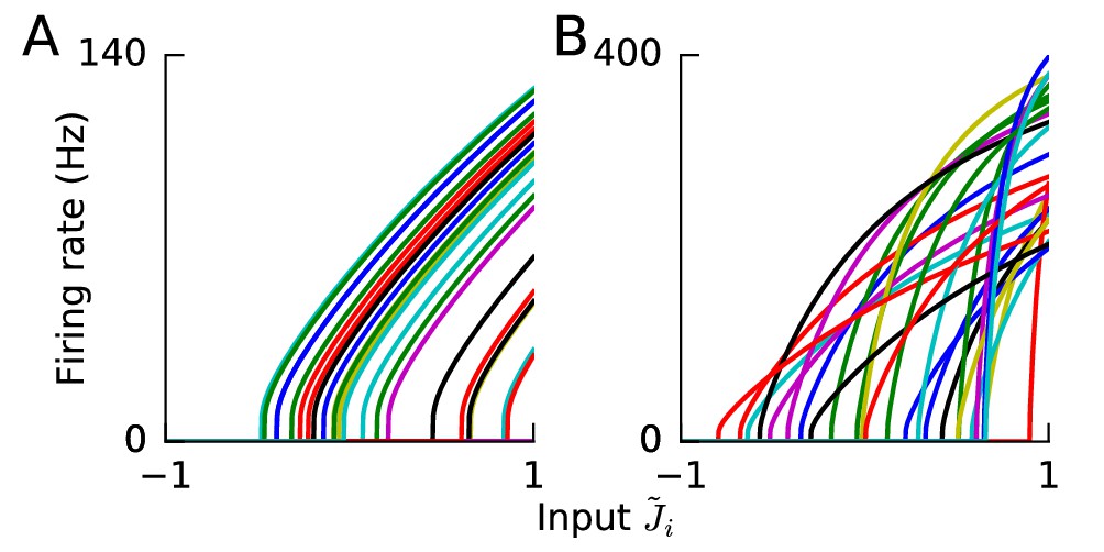
Gain functions of heterogeneous neurons.
The neurons in the command representation layer and the recurrent network were heterogeneous with different gain functions due to different gains and biases. (A,B) Illustrative gain functions of a few neurons as a function of (cf. Equation (13). The x-intercept is the rheobase input . (A) Neurons with constant gain used in Figure 2. (B) Neurons with firing rate uniformly between 200 and 400 Hz at , used in all other simulations (cf. Figure 2—figure supplement 1).
Figure 2 with 5 supplements
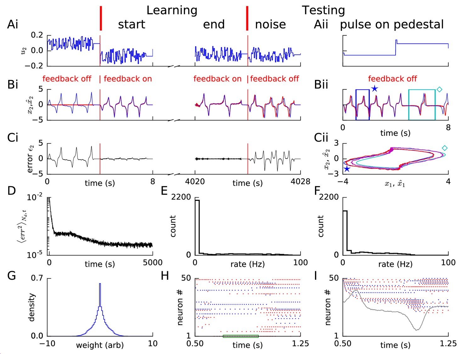
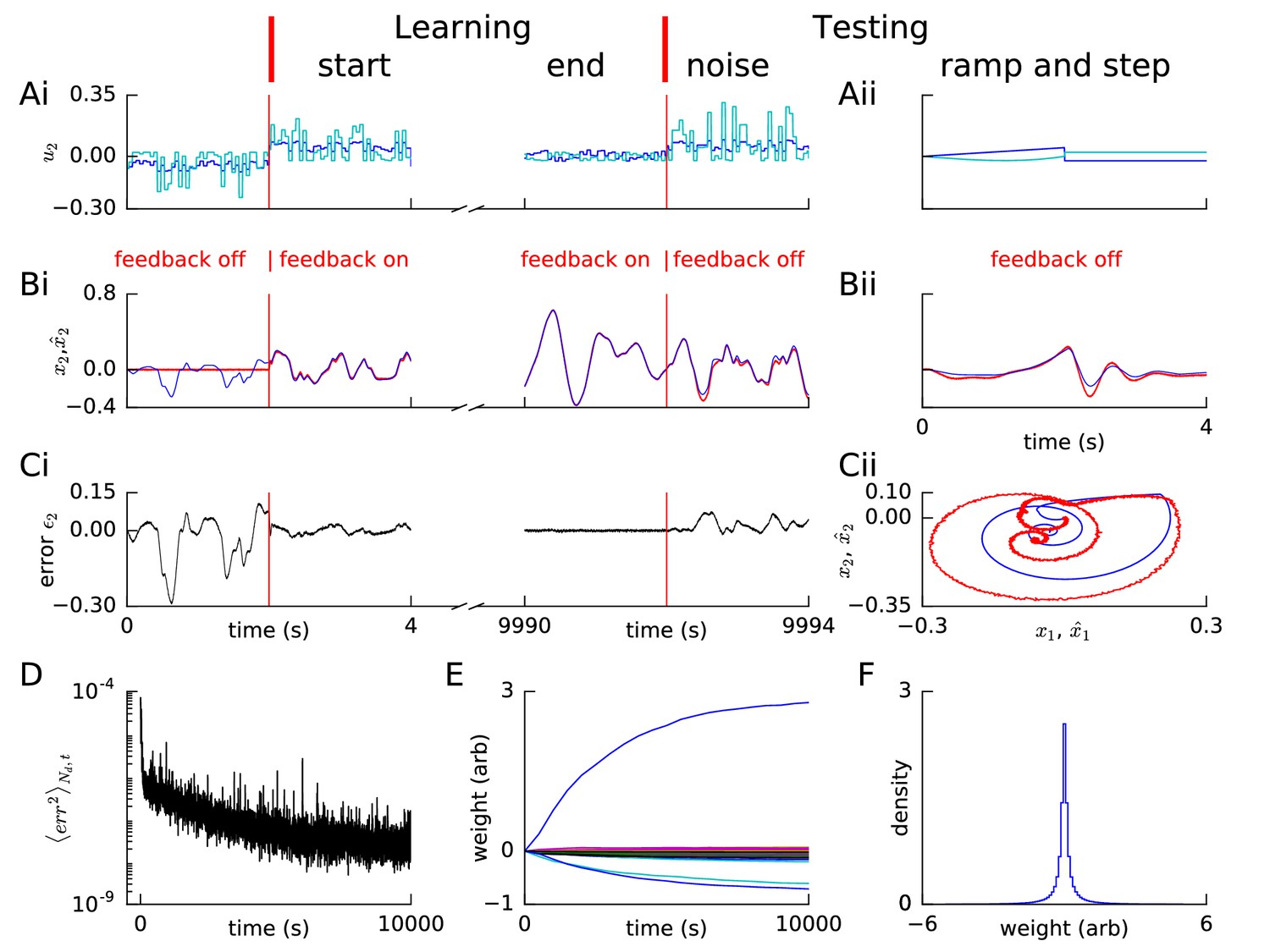
Learning non-linear dynamics via FOLLOW: the van der Pol oscillator.
(A-C) Control input, output, and error are plotted versus time, before the start of learning; in the first 4 s and last 4 s of learning; and during testing without error feedback (demarcated by the vertical red lines). Weight updating and error current feedback were both turned on after the vertical red line on the left at the start of learning, and turned off after the vertical red line in the middle at the end of learning. (A) Second component of the input . (B) Second component of the learned dynamical variable (red) decoded from the network, and the reference (blue). After the feedback was turned on, the output tracked the reference. The output continued to track the reference approximately, even after the end of the learning phase, when feedback and learning were turned off. The output tracked the reference approximately, even with a very different input (Bii). With higher firing rates, the tracking without feedback improved (Figure 2—figure supplement 1). (C) Second component of the error between the reference and the output. (Cii) Trajectory in the phase plane for reference (red,magenta) and prediction (blue,cyan) during two different intervals as indicated by and in Bii. (D) Mean squared error per dimension averaged over 4 s blocks, on a log scale, during learning with feedback on. Learning rate was increased by a factor of 20 after 1,000 s to speed up learning (as seen by the sharp drop in error at 1000 s). (E) Histogram of firing rates of neurons in the recurrent network averaged over 0.25 s (interval marked in green in H) when output was fairly constant (mean across neurons was 12.4 Hz). (F) As in E, but averaged over 16 s (mean across neurons was 12.9 Hz). (G) Histogram of weights after learning. A few strong weights are out of bounds and not shown here. (H) Spike trains of 50 randomly-chosen neurons in the recurrent network (alternating colors for guidance of eye only). (I) Spike trains of H, reverse-sorted by first spike time after 0.5 s, with output component overlaid for timing comparison.
Figure 2—figure supplement 1
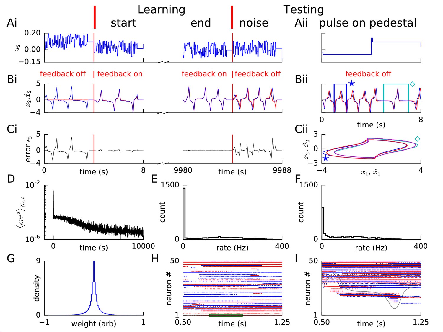
Learning van der Pol oscillator dynamics via FOLLOW with higher firing rates.
Layout and legend of panels A-I are analogous to Figure 2A–I, except that maximum firing rates of neurons were larger (Figure 1—figure supplement 1) yielding approximately seven times the mean firing rates (for panels E and F, mean over 0.25 s and 16 s was 86.6 Hz and 87.6 Hz respectively), but approximately one-eighth the learning time, with constant learning rate.
Figure 2—figure supplement 2
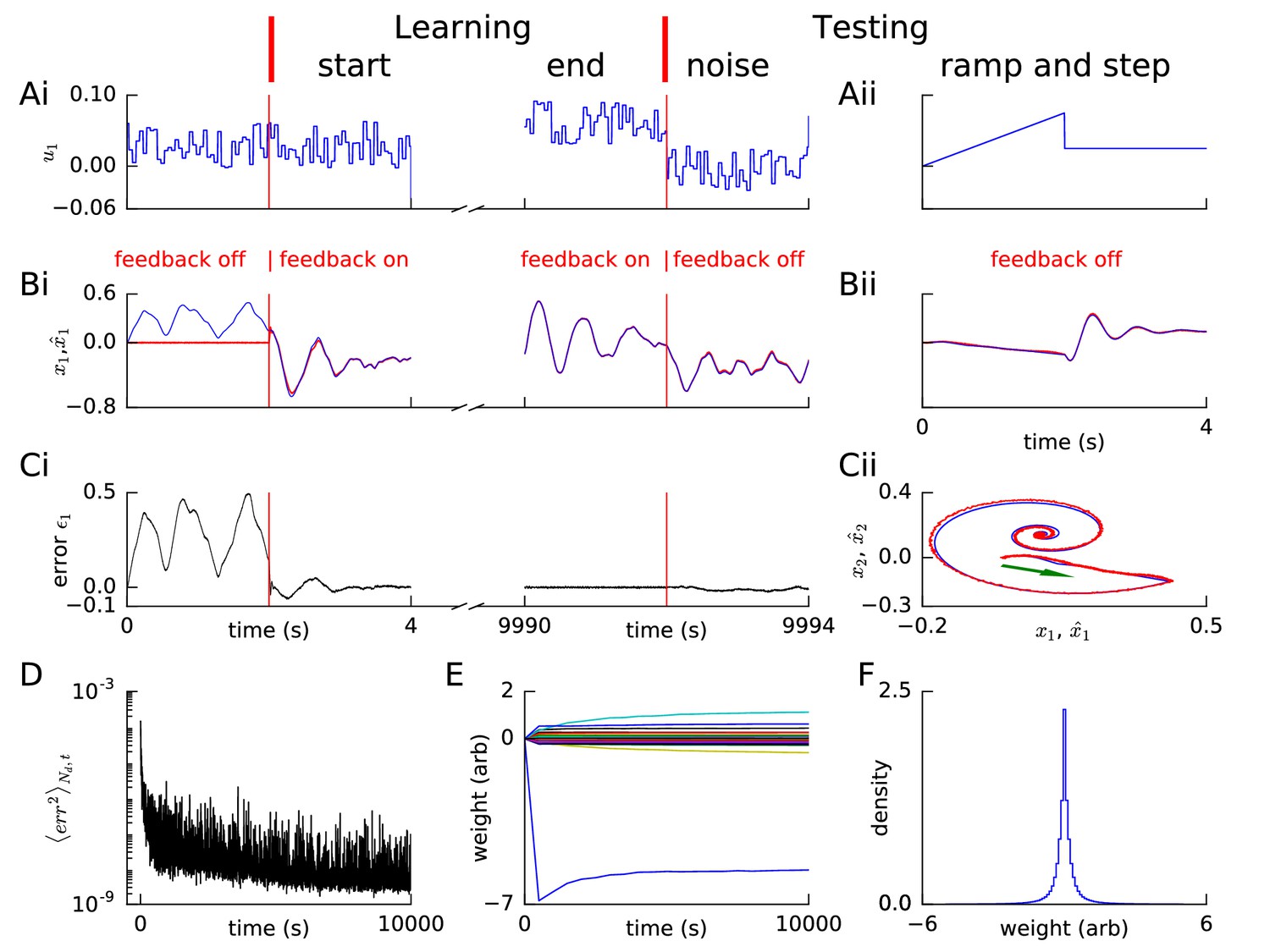
Learning linear dynamics via FOLLOW: 2D decaying oscillator.
Layout and legend of panels (A-D) are analogous to Figure 2A–D, the green arrow in panel Cii shows the start of the trajectory of Bii. (E) A few randomly selected weights are shown evolving during learning. (F) Histogram of weights after learning. A few strong weights are out of bounds and not shown here (cf. panel E).
Figure 2—figure supplement 3
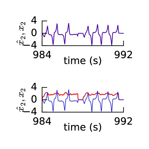
Readout weights learn if recurrent weights are as is, but not if shuffled.
(A-B) The readout weights were learned with a perceptron learning rule with the recurrent weights (A) as is after FOLLOW learning, or (B) shuffled after FOLLOW learning. A component of the output of the original FOLLOW-learned network (blue) and of the output of the network whose readout weights were trained (red) are plotted after the readout weights were trained for approximately 1,000 s. The readout weights learned if the recurrent weights were kept as is, but not if shuffled. Readout weights could also not be learned after shuffling only feedforward, and shuffling both feedforward and recurrent connections.
Figure 2—figure supplement 4
Learning non-linear feedforward transformation with linear recurrent dynamics via FOLLOW.
Panels A-F are interpreted similar to Figure 2—figure supplement 2A–F, except in panel A, along with the input (blue) to layer 1, the required non-linear transform is also plotted (cyan); and in panels E and F, the evolution and histogram of weights are those of the feedforward weights, that perform the non-linear transform on the input.
Figure 2—figure supplement 5
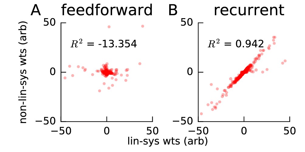
Feedforward weights are uncorrelated, while recurrent ones are correlated, when learning same recurrent dynamics but with different feedforward transforms.
The linear decaying oscillators system was learned for 10,000 s with either a non-linear or a linear feedforward transform. (A) The learned feedforward weights were plotted for the system with the non-linear feedforward transform, versus the corresponding feedforward weights for the system with the linear feedforward transform. The feedforward weights for the two systems do not fit the identity line (coefficient of determination is negative; is not the square of a number and can be negative) showing that the learned feedforward transform is different in the two systems as expected. (B) Same as A, but for the recurrent weights in the two systems. The weights fit the identity line with an close to one showing that the learned recurrent transform is similar in the two systems as expected. Some weights fall outside the plot limits.
Figure 3 with 1 supplement
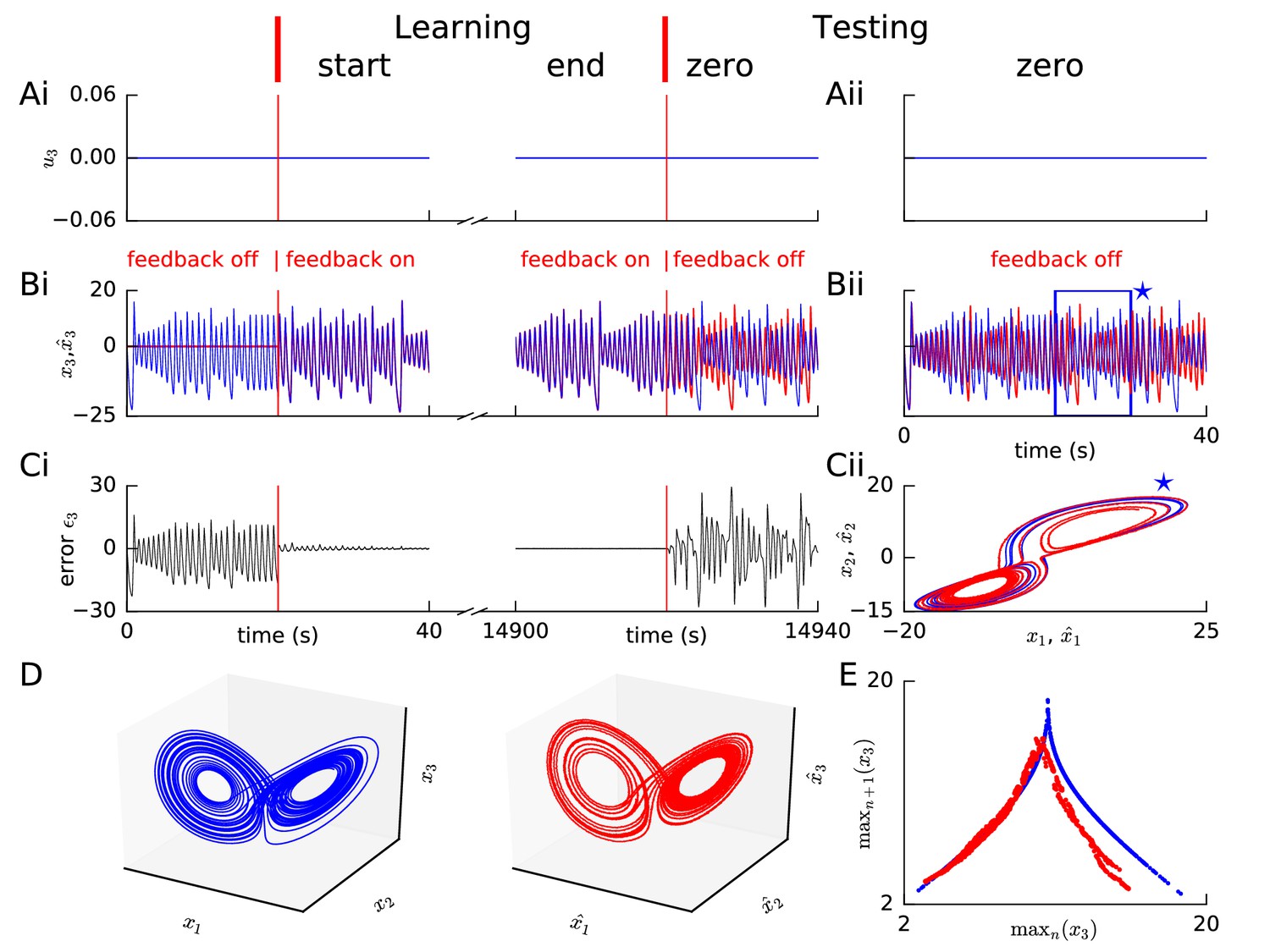
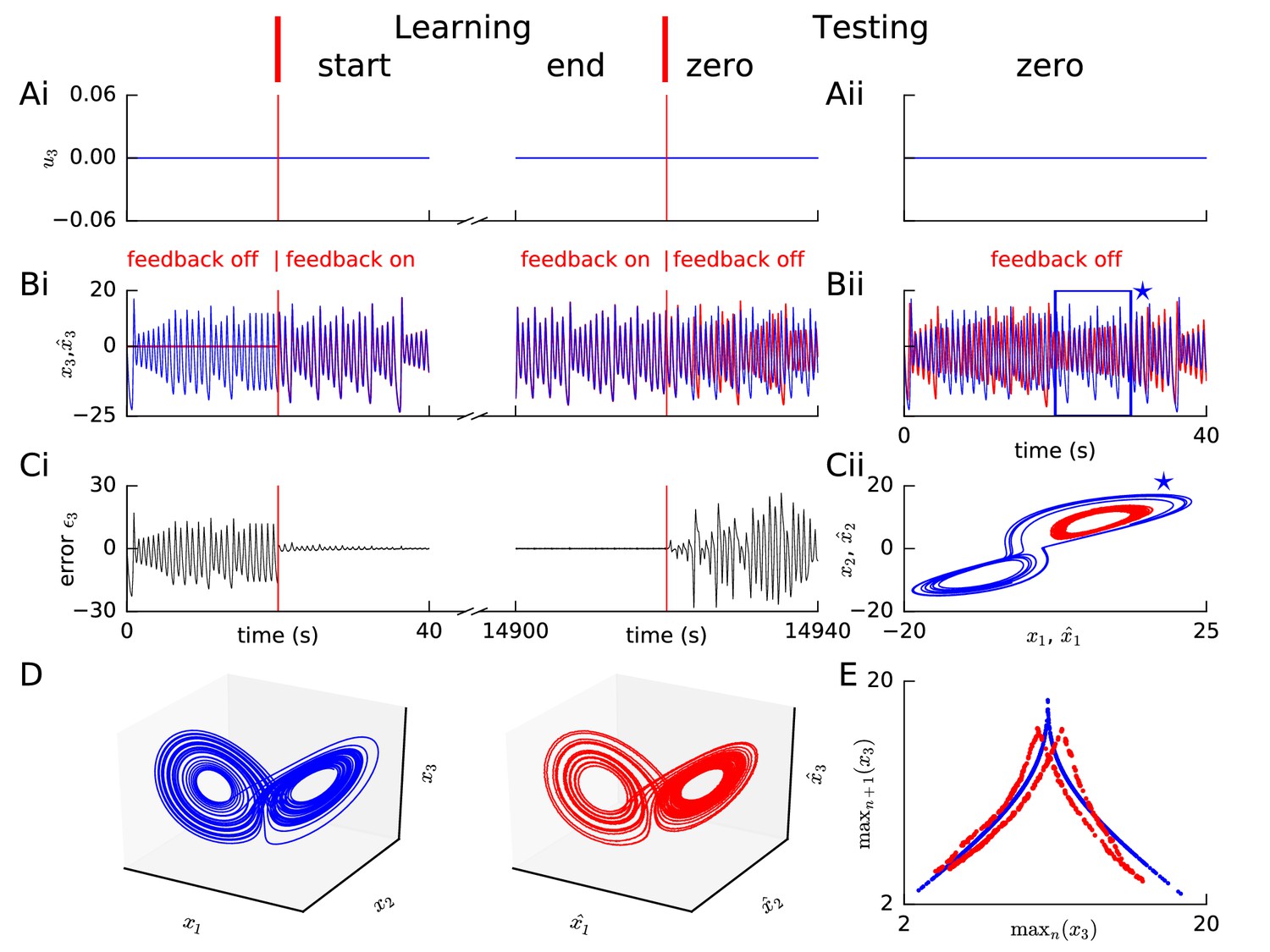
Learning chaotic dynamics via FOLLOW: the Lorenz system.
Layout and legend of panels (A-C) are analogous to Figure 2A–C. (D) The trajectories of the reference (left panel) and the learned network (right panel) are shown in state space for 40 s with zero input during the testing phase, forming the well-known Lorenz attractor. (E) Tent map, that is local maximum of the third component of the reference signal (blue)/network output (red) is plotted versus the previous local maximum, for 800 s of testing with zero input. The reference is plotted with filtering in panels (A-C), but unfiltered for the strange attractor (panel D left) and the tent map (panel E blue).
Figure 3—figure supplement 1
Learning the Lorenz system without filtering the reference variables.
Panels A-E are interpreted similar to Figure 3A–E, except that the reference signal was not filtered in computing the error. Without filtering, the tent map for the network output (panel E red) shows a doubling, but the mismatch for large maxima is reduced, compared to with filtering in Figure 3.
Figure 4

Learning arm dynamics via FOLLOW.
Layout and legend of panels A-C are analogous to Figure 2A–C except that: in panel (A), the control input (torque) on the elbow joint is plotted; in panel (B), reference and decoded angle (solid) and angular velocity (dotted) are plotted, for the elbow joint; in panel (C), the error in the elbow angle is plotted. (Aii-Cii) The control input was chosen to perform a swinging acrobot-like task by applying small torque only on the elbow joint. (Cii) The shoulder angle is plotted versus the elbow angle for the reference (blue) and the network (red) for the full duration in Aii-Bii. The green arrow shows the starting direction. (D) Reaching task. Snapshots of the configuration of the arm, reference in blue (top panels) and network in red (bottom panels) subject to torques in the directions shown by the circular arrows. After 0.6 s, the tip of the forearm reaches the cyan target. Gravity acts downwards in the direction of the arrow. (E) Acrobot-inspired swinging task (visualization of panels of Aii-Cii). Analogous to D, except that the torque is applied only at the elbow. To reach the target, the arm swings forward, back, and forward again.
Figure 5
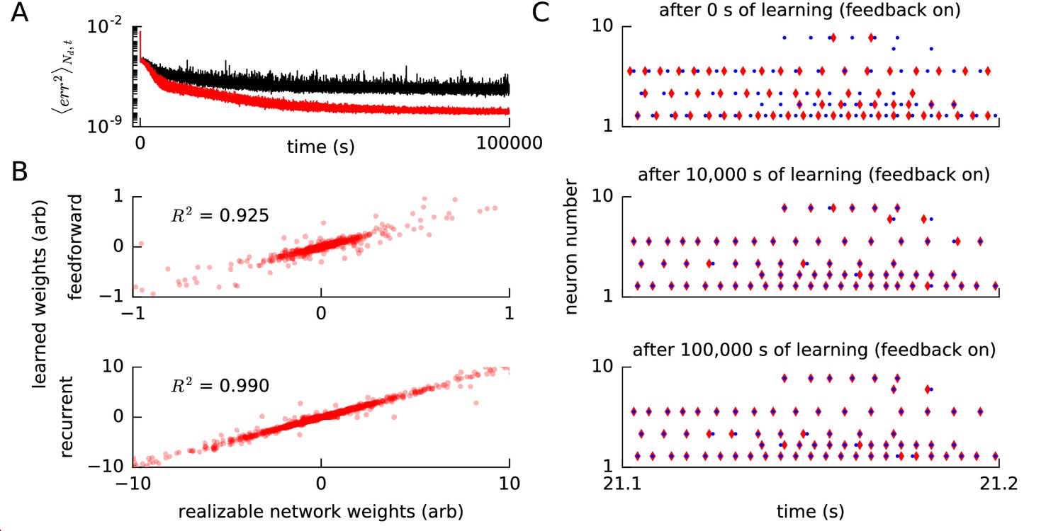
Convergence of error, weights and spike times for a realizable reference network.
(A) We ran our FOLLOW scheme on a network for learning one of two different implementations of the reference van der Pol oscillator: (1) differential equations, versus (2) a network realized using FOLLOW learning for 10,000 s (3 hr). We plot the evolution of the mean squared error, mean over number of dimensions and over 4 s time blocks, from the start to 100,000 s of learning, with the weights starting from zero. Mean squared error for the differential equations reference (1) is shown in black, while that for the realizable network reference (2) is in red. (B) The feedforward weights (top panel) and the recurrent weights (bottom panel) at the end of 100,000 s (28 hr) of learning, are plotted versus the corresponding weights of the realizable target network. The coefficient of determination i.e the value of the fit to the identity line () is also displayed for each panel. A value of denotes perfect equality of weights to those of the realizable network. Some weights fall outside the plot limits. (C) After 0 s, 10,000 s (3 hr), and 100,000 s (28 hr) of the learning protocol against the realizable network as reference, we show spike trains of a few neurons in the recurrent network (red) and the reference network (blue) in the top, middle and bottom panels respectively, from test simulations while providing the same control input and keeping error feedback on. With error feedback off, the low-dimensional output diverged slightly from the reference, hence the spike trains did too (not shown).
Figure 6

Robustness of FOLLOW learning.
We ran the van der Pol oscillator (A–D) or the linear decaying oscillator (F,H) learning protocol for 10,000 s for different parameter values and measured the mean squared error, over the last 400 s before the end of learning, mean over number of dimensions and time. (A) We evolved only a fraction of the feedforward and recurrent connections, randomly chosen as per a specific connectivity, according to FOLLOW learning, while keeping the rest zero. The round dots show the mean squared error for different connectivity after a 10,000 s learning protocol (default connectivity = 1 is starred); while the square dots show the same after a 20,000 s protocol. (B) Mean squared error after 10,000 s of learning versus the standard deviation of noise added to each component of the error, or equivalently to each component of the reference, is plotted. (C) We multiplied the original decoding weights (that form an auto-encoder with the error encoders) by a random factor (1 + uniform) drawn for each weight. The mean squared error at the end of a 10,000 s learning protocol for increasing values of is plotted (default is starred). (D) We multiplied the original decoding weights by a random factor (1 + uniform), fixing , drawn independently for each weight. The mean squared error at the end of a 10,000 s learning protocol, for a few values of on either side of zero, is plotted. (E,G) Architectures for learning the forward model when the reference is available after a sensory feedback delay for computing the error feedback. The forward model may be trained without a compensatory delay in the motor command path (E) or with it (G). (F,H) Mean squared error after 10,000 s of learning the linear decaying oscillator is plotted (default values are starred) versus the sensory feedback delay in the reference, for the architectures without and with compensatory delay, in F and H respectively.
Figure 7
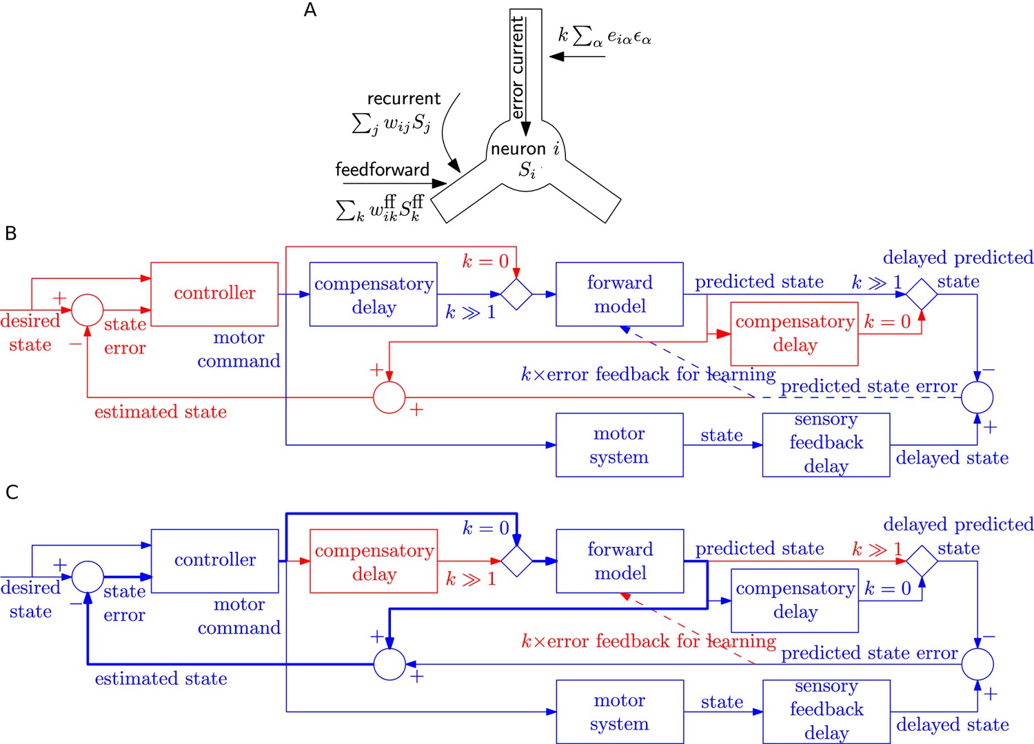
Possible implementation of learning rule, and delay compensation using forward model.
(A) A cartoon depiction of feedforward, recurrent and error currents entering a neuron in the recurrent network. The error current enters the apical dendrite and triggers an intra-cellular chemical cascade generating a signal that is available at the feedforward and recurrent synapses in the soma and basal dendrites, for weight updates. The error current must trigger a cascade isolated from the other currents, here achieved by spatial separation. (B-C) An architecture based on the Smith predictor, that can switch between learning the forward model (B), versus using the forward model for motor control (C, adapted from (Wolpert and Miall, 1996)), to compensate for the delay in sensory feedback. Active pathways are in blue and inactive ones are in red. (B) The learning architecture (blue) is identical to Figure 6G, but embedded within a larger control loop (red). During learning, when error feedback gain , the motor command is fed in with a compensatory delay identical to the sensory feedback delay. Thus motor command and reference state are equally delayed, hence temporally matched, and the forward model learns to produce the motor system output for given input. (C) Once the forward model is learned, the system switches to motor control mode (feedback gain ). In this mode, the forward model receives the present motor command and predicts the current state of the motor system, for rapid feedback to the controller (via loop indicated by thick lines), even before the delayed sensory feedback arrives. Of course the delayed sensory feedback can be further taken into account by the controller, by comparing it with the delayed output of the forward model, to better estimate the true state. Thus the forward model learned as in B provides a prediction of the state, even before feedback is received, acting to compensate for sensory feedback delays in motor control.
Videos
Video 1
Reaching by the reference arm is predicted by the network.
After training the network as a forward model of the two-link arm under gravity as in Figure 4, we tested the network without feedback on a reaching task. Command input was provided to both joints of the two-link reference arm so that the tip reached the cyan square. The same command input was also provided to the network without error feedback. The state (blue, left) of the reference arm and the state predicted (red, right) by the learned network without error feedback are animated as a function of time. The directions of the circular arrows indicate the directions of the command torques at the joints. The animation is slowed compared to real life.
Video 2
Acrobot-like swinging by the reference arm is predicted by the network.
After training the network as a forward model of the two-link arm under gravity as in Figure 4, we tested the network without feedback on a swinging task analogous to an acrobot. Command input was provided to the elbow joint of the two-link reference arm so that the tip reached the cyan square by swinging. The same command input was also provided to the network without error feedback. The state (blue, left) of the reference arm and the state predicted (red, right) by the learned network without error feedback are animated as a function of time. The directions of the circular arrows indicate the directions of the command torques at the joints. The animation is slowed compared to real life.
Tables
Table 1
Network and simulation parameters for example systems.
* 4e-2 after 1,000 s for Figures 1 and 2. 1e-4 for readout weights in Figure 2—figure supplement 3.
Nengo v2.4.0 sets the gains and biases indirectly, by default. The projected input at which the neuron just starts firing (i.e. ) is chosen uniformly from , while the firing rate for is chosen uniformly between 200 and 400 Hz. From these, and are computed using Equations (11) and (13).
| Linear | Van der pol | Lorenz | Arm | Non-linear feedforward | |
|---|---|---|---|---|---|
| Number of neurons/layer | 2000 | 3000 | 5000 | 5000 | 2000 |
| (s) | 2 | 4 | 20 | 2 | 2 |
| Representation radius | 0.2 | 0.2 | 6 | 0.2 | 0.2 |
| Representation radius | 1 | 5 | 30 | 1 | 1 |
| Gains and biases for command representation and recurrent layers | Nengo v2.4.0 default | Figures 1 and 2: and chosen uniformly from . all other Figures: Nengo v2.4.0 default | Nengo v2.4.0 default | Nengo v2.4.0 default | Nengo v2.4.0 default |
| Learning pulse | |||||
| Learning pedestal | , | 0 | |||
| Learning rate | 2e-3 | 2e-3* | 2e-3 | 2e-3 | 2e-3 |
| Figures | Figure 2—figure supplement 2 | Figure 1, Figure 2, Figure 2—figure supplement 1, Figure 2—figure supplement 3, Figure 5, Figure 6, Figure 7 | Figure 3, Figure 3—figure supplement 1 | Figure 4 | Figure 2—figure supplement 4, Figure 2—figure supplement 5 |
Additional files
-
Transparent reporting form
- https://doi.org/10.7554/eLife.28295.019
Download links
A two-part list of links to download the article, or parts of the article, in various formats.
Downloads (link to download the article as PDF)
Open citations (links to open the citations from this article in various online reference manager services)
Cite this article (links to download the citations from this article in formats compatible with various reference manager tools)
Predicting non-linear dynamics by stable local learning in a recurrent spiking neural network
eLife 6:e28295.
https://doi.org/10.7554/eLife.28295


