Cell-accurate optical mapping across the entire developing heart
- Max Planck Institute of Molecular Cell Biology and Genetics, Germany
- Harvard Medical School, United States
- Max Planck Institute for Human Cognitive and Brain Sciences, Germany
- Max-Delbrück-Center for Molecular Medicine in the Helmholtz Association, Germany
- DZHK (German Centre for Cardiovascular Research), Germany
- University Heart Centre Freiburg - Bad Krozingen, Faculty of Medicine, Albert-Ludwigs University, Germany
- Morgridge Institute for Research, United States
Figures
Figure 1 with 9 supplements

In vivo 3D optical mapping reveals cell-specific calcium transient patterns at 52 hr post fertilization (hpf).
(a) Transmitted light microscopy image with ~250 µm-sized, two-chambered heart (shown as fluorescence image with light sheet illumination path). (b) Genetically encoded fluorescent markers expressed in myocardial cells report calcium transient activity and cell positions. Volumetric movies were reconstructed from multiple high-speed movies, each with a temporal resolution of 2.5 ms and a voxel size of 0.5 µm in xy and 1 µm in z. Image data are available at Weber et al. (2017). (c’) Normalized fluorescence plot of every cell’s calcium transient over one cardiac cycle. The network’s activation timing (tact) is visualized in 3D based on the time-point of 10% calcium transient amplitude in every individual cell (right, same color scale). (c’’) Normalized fluorescence plot of all calcium transients, aligned in time based on the timing of deviation from minimal fluorescence intensity (3D network, same color scale). (d) Biological conduction speed, expressed as cells activated per unit of time, is visualized on the 3D network. (e) The basis vectors of the local coordinate system (tangent – black, normal – grey, and binormal – blue) are shown, moving along the centerline. The initial and final orientation of the moving reference frame is shown in a zoomed version at inflow and outflow sites. Outer curvature regions of atrium and ventricle are highlighted in green. (f) The unrolled cylinder results in a representation of 3D network function in a 2D map. Projections show conduction speed across the entire myocardium; iso-velocity lines (Δv = 50 cells/s) are shown in black. Outer curvature regions in atrium and ventricle are highlighted in green.
Figure 1—figure supplement 1

High-speed light sheet microscopy for in vivo 3D optical mapping.
(A) A zebrafish embryo is mounted in agarose inside a fluorinated ethylene propylene (FEP) tube. (B) Section view of the sample holder with mounted zebrafish embryo placed inside the medium-filled sample chamber. The embryo is placed in the field of view of the detection objective and illuminated with a static light sheet from one of two sides. (C) Top view of the high-speed light sheet microscope for in vivo cardiac imaging. The laser module combines a 488 and a 561 nm laser line and sends the beam into the two illumination arms. Both arms generate identical light sheets from two opposite sides. The motor unit positions the sample holder with the mounted zebrafish embryo at the intersection of illumination and detection path. Fluorescence emission is split and recorded with an sCMOS camera running at up to 400 Hz.
Figure 1—figure supplement 2
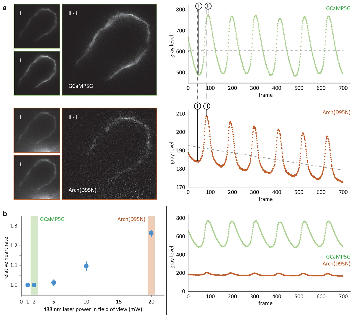
Comparison of the calcium reporter GCaMP5G and the voltage reporter Arch(D95N) for multi-scale readout of cardiomyocyte activation.
(a) Optical section across the atrium of a zebrafish embryo at 52 hpf expressing GCaMP5G and Arch(D95N) in cardiomyocytes. Both channels are recorded simultaneously. Smaller images: raw data recorded at the lowest (I) and highest (II) fluorescence signal, as indicated in the intensity plots. Note how intensity plots illustrate the known slight delay between intensity maxima of calcium versus voltage traces, and the overall excellent capture by both reporters of presence and temporal dynamics of cell activation. Larger images: results of image I subtracted from image II, presenting the maximum intensity difference (image brightness adjusted independently for better visibility). Plots show mean raw intensities over time measured along the myocardium visible in the images. (b) Laser powers in the field of view (measured at the back pupil of the illumination objective) used for the experiment presented in (a) and their impact on the heart rate (n = 3 zebrafish embryos). Arch(D95N) required 10x more laser power than GCaMP5G, yielded a very low signal with about 20 gray levels dynamic range across one cardiac cycle, and was affected by bleaching. Zebrafish embryos showed increased heart rate when illuminated with the high laser power needed for Arch(D95N) imaging. GCaMP5G showed a dynamic range of about 300 gray levels at an order of magnitude lower laser power, with no signs of visible photobleaching or illumination-induced increase in heart rate.
Figure 1—figure supplement 3
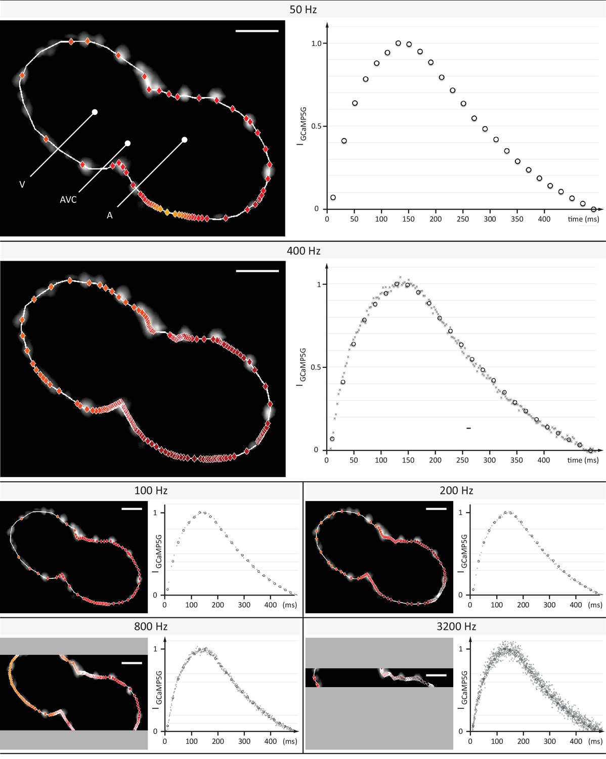
Evaluation of signal coverage and tracing precision using the fluorescent calcium reporter GCaMP5G at different recording speeds.
Optical sections across the silenced heart of a 2 days post fertilization (dpf) zebrafish embryo expressing GCaMP5G and H2A-mCherry in cardiomyocytes, recorded at 50 to 3200 Hz (exposure times 20 to 0.3 ms) with a constant pixel size of (0.5 µm)2. Raw image data of H2A-mCherry are shown to mark cell positions. Red markers indicate location of peak fluorescence intensities across a single cardiac cycle. Gray areas in 800 Hz and 3200 Hz images indicate the proportion of the field of view that could not be recorded, as the number of lines imaged is the speed-limiting factor on the sCMOS camera. Plots show normalized fluorescence intensity over time, measured in a sub region with GCaMP5G signal. Circles show data points from the measurement at 50 Hz as reference. Higher recording speed results in a better representation of the calcium transient until 400–800 Hz, especially during the initial rise in intensity. At an even higher rate of 3200 Hz, noise deteriorates the signal. Peak intensities could be traced with cellular precision at 400 and 800 Hz, before signal noise reduced precision.
Figure 1—figure supplement 4
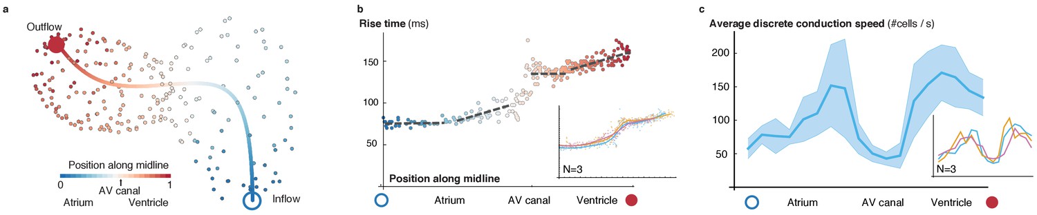
Activation and conduction properties of cells vary from inflow to outflow, with patterns conserved across different hearts (52 hpf, n = 3).
(a) The centerline is traced in 3D from inflow (blue) to outflow (red), providing the base for a canonical ordering of the cells. Color code indicates position of cell along midline. (b) Populations of cells with different rise times can be distinguished close to the inflow tract, in the atrium and in the ventricle (indicated by different linear fits), with a pronounced discontinuity in the atrio-ventricular canal (AVC). Color code indicates position of cell along midline. (c) Distribution of biological conduction speeds across the heart, from inflow (blue circle) to outflow (red disk), mean and standard deviation. The inset shows the mean conduction speed for three different hearts at 52 hpf.
Figure 1—figure supplement 5
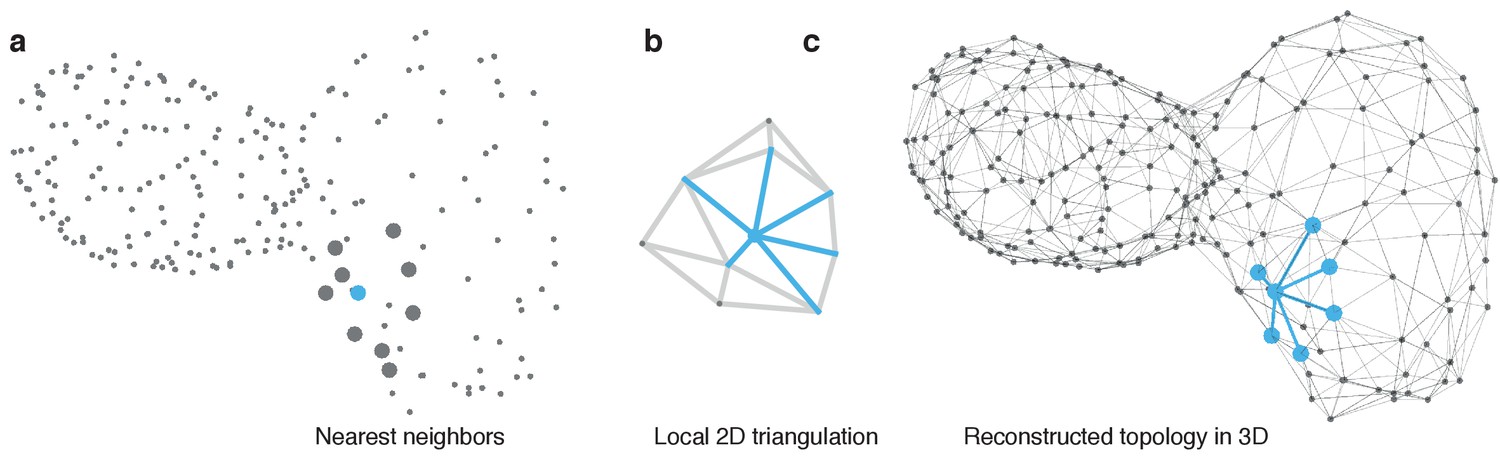
Reconstruction of myocardial topology.
(a) Cell positions are indicated by points at the optically identified location of their nucleus in 3D. Potential neighbors for each cell are identified by taking nearest neighbors with respect to their Euclidean distance in 3D. A sample cell is highlighted in blue and the respective nearest neighbors by large gray dots. (b) The centroids are locally projected into a 2D plane and the Delaunay triangulation (gray and blue lines) is computed to extract the topological connectivity between cells. Edges connecting the reference cell with its neighbors in the 2D projection are highlighted in blue. (c) The connections between the reference cell and its neighbors (blue) are projected back into the original 3D space. Iterating this procedure for all cells yields the final topology (gray edges).
Figure 1—figure supplement 6
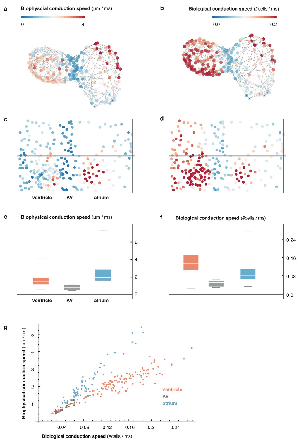
Comparison of metric and cell-to-cell speed measurements.
(a) Biophysical conduction speed, expressed in μm/ms, is visualized on the 3D network. (b) Visualization of biological conduction speed, expressed as cells activated per unit of time (ms) on the same topology as (a). (c, d) Projection show biophysical (c) and biological (d) conduction speed across the entire myocardium. Same color code as in (a, b). (e, f) Descriptive statistics of conduction speeds in (manually defined) regions corresponding to atrial (blue), AVC (gray), and ventricular part (orange) of myocardium for biophysical (e) and biological (f) conduction speed. (g) Scatterplot showing chamber-specific differences in correlation of biological (x-axis) vs. biophysical (y-axis) conduction speed for atrial (blue), AVC (gray) and ventricular (orange) cells.
Figure 1—figure supplement 7
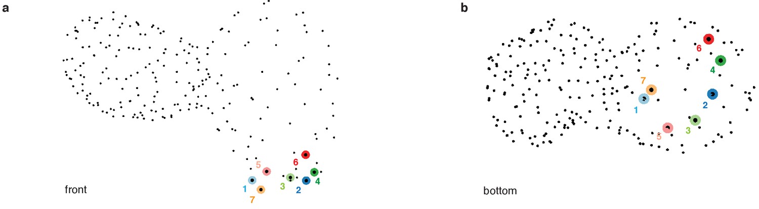
Location of pacemaker cells.
(a, b) Pacemaker cells (shown as colored disks), are located in a ring-like region at the atrial inflow region, shown in front (a) and bottom view (b).
Figure 1—figure supplement 8
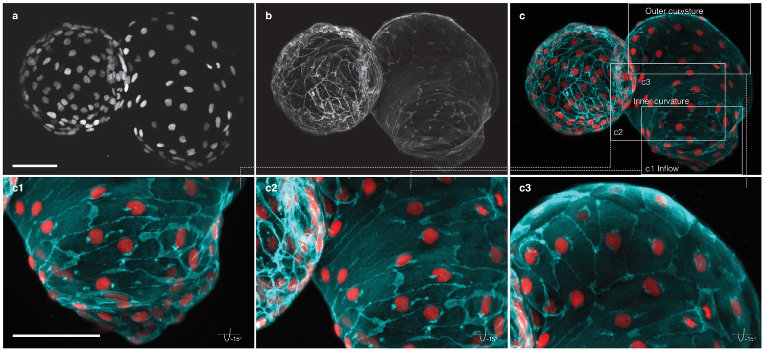
Myocardial morphology is heterogeneous across the heart at 52 hpf.
Maximum intensity projections of point-scanning confocal and two-photon microscopy z-stacks recorded from a transgenic zebrafish embryo expressing myl7:H2A-mCherry and myl7:lck-EGFP in the myocardium. Scale bars: 50 µm. (a) Positions of myocardial nuclei (myl7:H2A-mCherry) across the heart. (b) Myocardial cell membranes (myl7:lck-EGFP). (c) Color overlay of cell membranes (cyan) and nuclei (red). (c1-3) Detailed view (rotated by −15 degrees about x–axis) of the cell morphologies in inflow, inner curvature and outer curvature regions of the atrium, as indicated in panel (c).
Figure 1—figure supplement 9
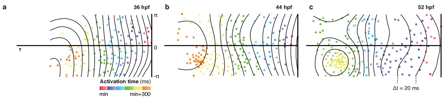
Patterns of cell activation across myocardium.
Global distribution of cellular activation times shown as 2D projections, illustrate planar activation in spite of increasingly complex chamber morphology and heterogeneity in individual cell properties. Isochronal lines shown in black (Δt = 20 ms).
Figure 2 with 3 supplements

Organ maturation and functional cell remodelling from 36 to 52 hpf.
(a–c) Normalized calcium transients of all cells are shown at three different time-points: (a) 36, (b) 44, and (c) 52 hpf. The shortening of black arrows indicates the decrease in time between earliest and latest activation of cells along the whole heart. The gradual formation of atrial (1) and ventricular (2) populations with increasingly different calcium transients is highlighted by the dashed lines at 52 hpf. The color of each transient indicates its activation time (all three plots use the same color scale). (d–f) Changes in cardiac and cellular morphology at each developmental time point. Estimated cell shapes are visualized as scaled ellipsoids. The color of each ellipsoid indicates activation time (relative to the first-activated cell); color code as in (a–c). Two main populations of cells corresponding to highlighted clusters in (c) are indicated by numbers. (g–i) 3D pattern of biological conduction speeds across the heart. The formation of outer curvature clusters of cells over time is highlighted by arrows. (j–l) Development of conduction speeds across the myocardium, shown as 2D projections for the three time points. The color code indicates conduction speed. Isovelocity lines are shown in black (Δv = 50 cells/s). Corresponding outer curve cell populations are highlighted by arrows.
Figure 2—figure supplement 1
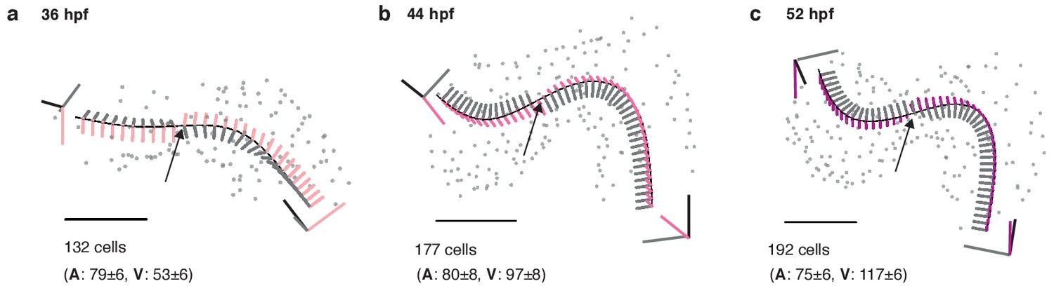
Structural organ maturation from 36 to 52 hpf.
(a) One and the same developing heart, imaged at three different time-points (36 (a), 44 (b), and 52 hpf (c), scale bar 50 μm. The fitted centerline visualizes the re-shaping of the myocardium during the ongoing looping/twisting process in early cardiac development. Local coordinate systems are shown along the midline (tangent – black, normal – grey, binormal – color), the twisting point is highlighted by an arrow. Total and chamber-specific cell numbers are indicated for each stage of development (A - atrial cells, V - ventricular cells).
Figure 2—figure supplement 2

Developmental changes of cellular characteristics along the heart.
(a) The distribution of activation times is shown for three time points: 36, 44 and 52 hpf. Dots indicate individual cell activation times. Smooth regression profiles are depicted as solid lines and show faster activation with progressive organogenesis. (b) The distribution of rise times during development. The probability density function of each developmental stage is shown by a smooth kernel density. The ordinate axis shows cell numbers and illustrates progressive emergence of cell sub-populations with different calcium transient properties. (c) The distribution of each cell’s conduction speed along the midline is shown as dots. Solid lines indicate smooth regression profiles for each stage. All hearts were normalized to a standard length, showing how speed of biological conduction in working myocardium rises by comparison with early developmental stages, whereas AVC conduction velocity is unchanged.
Figure 2—figure supplement 3

Cell shape changes during development.
Cell shapes in the atrium are represented by scaled ellipsoids for the same heart at 36 hpf (a), 44 hpf (b), and 52 hpf (c). Ventricular cells are shown with reduced opacity. (d, e, f) The same cells as in (a, b, c) with additional color code indicating cell size. Smaller cells are shown in blue, larger cells in red, highlighting the increase in cell size, in particular along the larger curvature of the atrium. Changes in cell size shown as 2D projections for 36 (g), 44 (h), and 52 hpf (i). The color code indicates normalized cell size as in (d, e, f). Isosize lines shown in black (ΔA = 0.1).
Videos
Video 1
Raw GCaMP5G signal at different imaging depths.
Fluorescence signal recorded at 400 Hz at three different depths (50, 90 and 140 μm along the optical axis) in the heart of a living Tg(myl7:GCaMP5G) zebrafish at 52 hpf using the described imaging setup.
Video 2
Calcium signal at different imaging depths after synchronization.
Raw data from Video 1 after completed post-acquisition synchronization.
Video 3
4D reconstruction of cellular calcium transients.
(1) 4D reconstruction of calcium activation from the synchronized planar movies recorded in the heart of a living Tg(myl7:GCaMP5G) zebrafish embryo at 52 hpf. The number of slices used in the reconstruction is indicated by n. Raw GCaMP5G signal is shown in orange. Time is indicated in ms. (2) Cell detection: The raw fluorescence signal of myl7:H2A-mCherry is overlaid with the centroids of detected nuclei. (3) Calcium mapping: The raw myl7:GCaMP5G signal is shown. The dots indicate the extracted cellular positions. (4) Cell-specific transients: The normalized GCaMP5G transients are shown for two sample cells (one atrial and one ventricular cell).
Video 4
Computation of biological conduction speed.
(1) Activation timing: Cell positions are indicated by gray dots. Activated cells are highlighted in yellow. Time is shown in ms. (2) Network reconstruction: Estimated local topology is shown as gray edges connecting neighboring cells. (3) Activation across network: Activated cells in the network are highlighted in yellow. (4) Cell–cell conduction speed: The average conduction speed is shown for each cell after activation of its neighbors in the network. Color code indicates conduction speed (red - high, blue - low).
Video 5
Mapping of myocardial geometry.
(1) Tracing of midline: The black line traces the center of the myocardium from inflow to outflow. Cellular positions are shown as gray spheres. (2) Moving reference frame: The intrinsic reference frame is shown along the extracted midline. The three axes represent the tangent (black), normal (gray), and binormal (blue) vectors. The trace of the binormal vector is shown as blue band behind the moving trihedron. (3) Untwisting: The heart is successively untwisted by reducing the torsion of the midline to 0. The gray lines indicate traces of cells during this process. (4) Straightening: The heart is straightened by reducing the remaining curvature of the midline to 0. (5) Projection to cylinder. Each cell is projected to the same radial distance from the straightened midline resulting in a cylindrical reference system. (6) Unrolling: The cylinder is unfolded into the 2D plane, resulting in the 2D plots used in the main text. Color code in the final frame indicates biological conduction speed.
Additional files
-
Transparent reporting form
- https://doi.org/10.7554/eLife.28307.022
Download links
A two-part list of links to download the article, or parts of the article, in various formats.
Downloads (link to download the article as PDF)
Open citations (links to open the citations from this article in various online reference manager services)
Cite this article (links to download the citations from this article in formats compatible with various reference manager tools)
Cell-accurate optical mapping across the entire developing heart
eLife 6:e28307.
https://doi.org/10.7554/eLife.28307


