Phasic and tonic neuron ensemble codes for stimulus-environment conjunctions in the lateral entorhinal cortex
Figures
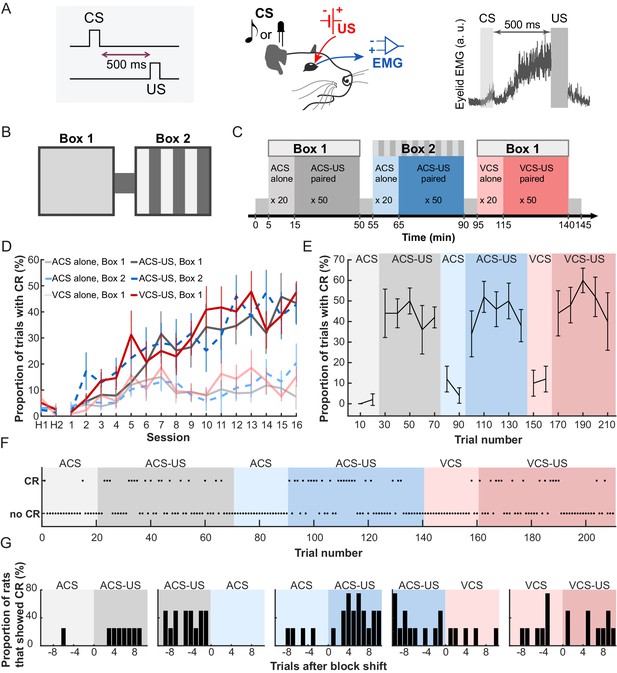
Rats acquired three associative memories with different stimulus and environmental features.
(A) In trace eyeblink conditioning, animals associated a neutral conditioned stimulus (CS) with electrical shock near the eyelid (US) over a temporal gap (500 ms). With repeated pairings, rats developed anticipatory blinking responses before US onset (CRs), which were monitored by recording electromyogram (EMG) from the upper eyelid (a.u., arbitrary unit). (B) Daily conditioning took place in a conditioning chamber which consisted of two visually distinct rooms (Box 1 and 2) connected by a short walkway. (C) Rats first entered Box 1 and received an auditory stimulus (ACS) alone for 20 trials (CS-alone block), followed by 50 ACS-US pairings (CS-US block). They then moved to Box 2, where they received 20 ACS alone trials followed by 50 ACS-US paired trials. Finally, they returned to Box 1 and received a visual stimulus (VCS) alone for 20 trials followed by pairings of the VCS and US for 50 trials. (D) The frequency of CR expression increased in the CS-US paired, but not in the CS-alone, trials (mean CR% ± SEM; n = 7 rats; Sessions × Trial blocks interaction, F75, 450 = 2.992, p<0.001). H1 and H2 show the rate of blinking when only the CS was presented before any conditioning. (E) In the last session, CR% (in every 10 trials, mean ± SEM; n = 5 rats that received the CS-alone block before the CS-US paired blocks) showed an abrupt transition upon the shift from the block of CS-alone trials (light colors) to the block of CS-US paired trials (dark colors). (F) A trial-by-trial pattern of CR expression of Rat 2 during the last session. (G) The proportion of rats (n = 4 rats underwent the trial blocks in the same temporal sequence) that showed the CR in each trial during the last session.
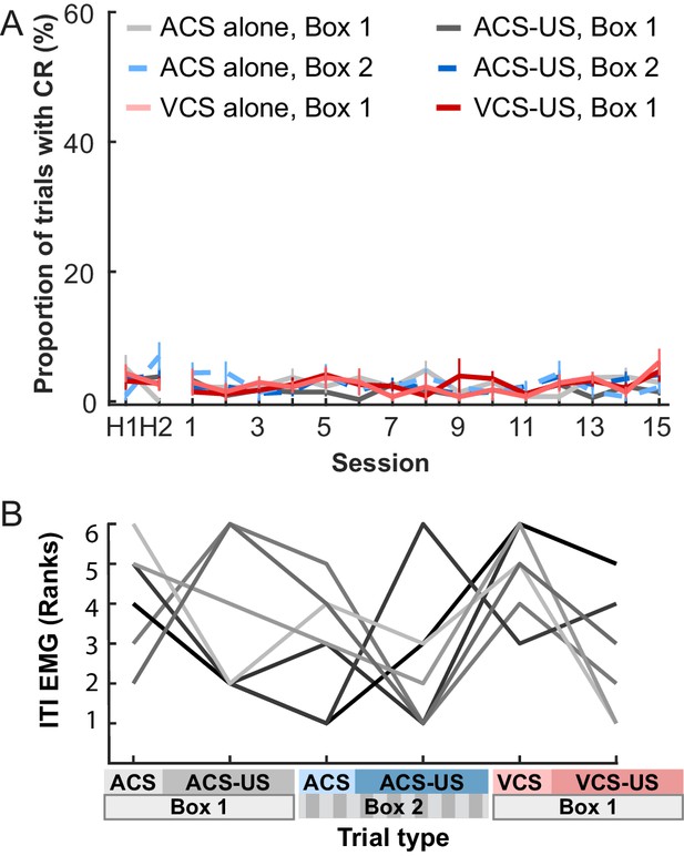
EMG activity during intervals between CS presentations.
(A) The proportion of trials with significant eyelid EMG amplitude change (pre-CRs) remained low across sessions and did not differ between CS-alone and CS-US paired trials (mean ± SEM; n = 7 rats; Sessions × Trial blocks interaction, F70, 420 = 8.482, p=0.717). (B) As a measure of the general activity level during each trial blocks, eyelid EMG amplitude was averaged across the entire period of a block and converted to ranks. The ranked amplitude (one line for each of seven rats) was comparable among six trial blocks (Kruskal-Wallis test, χ25 = 10.11, p=0.072).
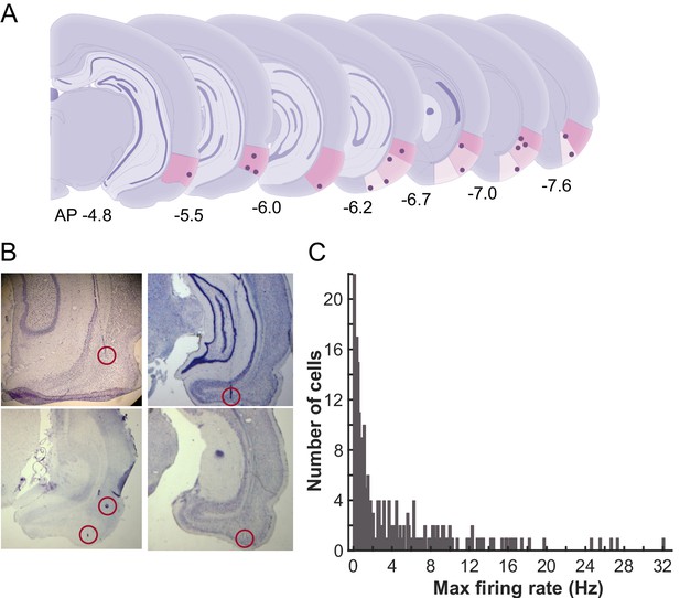
Recording locations and average firing rates of LEC units.
(A) Schematic representations of the recording sites in the LEC along the anterior-posterior axis. The dots indicate final locations of tetrodes. The numbers show the distance from bregma (mm) (B) Example photomicrographs of the Nissl stained coronal sections with the tracks and final locations of the tetrodes (circled). (C) Histogram of the averaged firing rate (FR) of the recorded LEC cells. In each cell, FRs during inter-trial intervals were separately calculated in six trial blocks, and the highest FR was used as the FR for a cell.
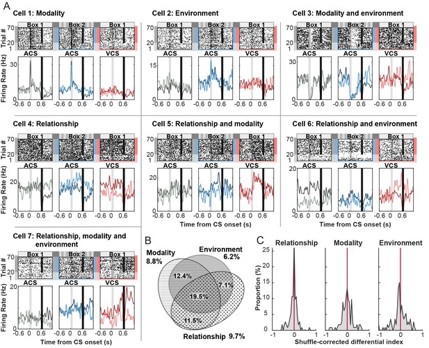
Phasic firing patterns selective for stimulus-environment conjunction.
(A) Examples of firing patterns of cells that were identified as selective for stimulus relationship (CS alone vs. CS-US paired, Relationship), stimulus modality (auditory vs. visual CS, Modality), or conditioning environment (Box 1 vs. 2, Environment) and their combinations. Rasters and peristimulus time histograms (PSTH) represent activity patterns during the presentations of one of two CS (auditory, ACS or visual, VCS) in one of two conditioning environments (Box 1 or 2). Time 0 indicates CS onset. In each PSTH, the lines in light color show the firing pattern to the CS presented alone (the first 20 trials) while those in dark color show the pattern to the CS paired with the US (the latter 50 trials). Light gray shadings indicate the CS, and black bars mask the artifact induced by the US. (B) Area-proportional three-venn diagram (Micallef and Rodgers, 2014) showing a major overlap in selective cells for three task variables. The numbers show the percentage of cells in each category to total CS-responding cells. (C) Distributions of shuffle-corrected differential indices. A positive value means the significant selectivity (random permutation tests, α = 0.05).
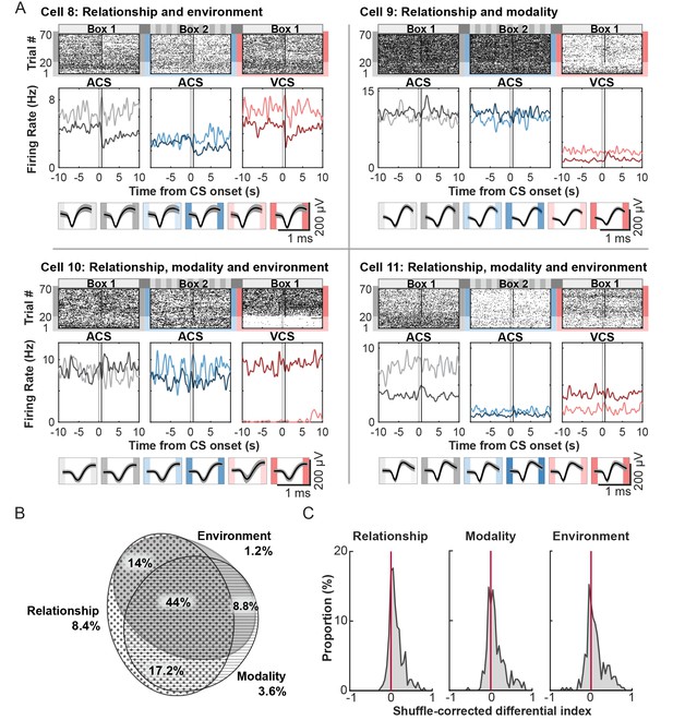
Tonic firing patterns selective for stimulus-environment conjunction.
(A) Examples of firing patterns of cells during intervals between trials with rasters and peristimulus time histograms as in Figure 3A. The bottom panel shows each cell’s average waveforms recorded in one of four wires of a tetrode during six trial blocks. (B) Area-proportional three-venn diagram showing that the majority of cells were selective for more than one task variable. The numbers show the percentage of cells in each category to all cells. (C) Distribution of the shuffle-corrected differential indices as in Figure 3C.
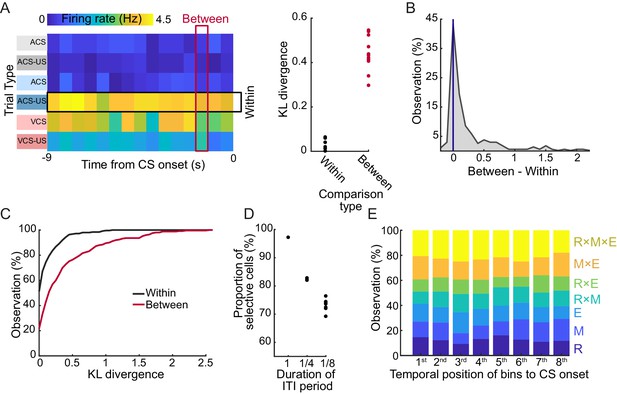
LEC cells stably maintained the selectivity for stimulus-environment conjunction during the stimulus-free period.
(A) Example of fluctuations of binned firing rates (FR) of a cell across the 9 s interval during each of six trial blocks. The degree of FR fluctuation was marginal across time bins in each trial block (‘Within’, rows) while FR greatly changed across six blocks (‘Between’, columns) as evident in the difference in Kullback-Leibler divergence from a uniform distribution (KLD, right). (B) Distribution of the difference between the Between-KLD and Within-KLD. (C) Cumulative distribution of the Within- (black) and Between- (red) KLD. (D) Difference in the proportion of cells whose ITI firing rates were judged as selective for at least one of three task features depending on the bin size. The same criteria were applied to averaged firing rates in one 9 s bin (1), four 2.25 s bins (1/4), or eight 1.125 s bins (1/8) covering the 9 s ITI. (E) The proportion of selectivity categories (see Table 4) of firing rates during a series of eight 1.125 s bins during the 9 s ITI. The 8th bin was the closest to CS onset.
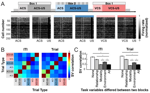
Ensemble activity showed a comparable level of selectivity for stimulus-environment conjunction during stimulus and non-stimulus periods.
(A) Grayscale plots show the normalized firing rate during six trial blocks (from left, ACS trials in Box 1, ACS-US trials in Box 1, ACS trials in Box 2, ACS-US trials in Box 2, VCS trials in Box 1, and VCS-US trials in Box 1). Cells were sorted based on the ACS-induced firing rate during the ACS-US block in Box 1, from the largest increase (cell #1) to the largest decrease (cell #250). Two white lines indicate the onset and offset of the CS while black bars mask US artifacts. (B) Matrices of the correlation coefficient (r) of ensemble firing rates (State vector, SV) between two of six trial blocks during CS-US pairings (Trial) and intervals between trials (ITI). (C) During both task phases, the r for two blocks with different CS (Modality; mean ± SEM, n = 20 runs with 10 subsampled trials) was comparable to that for two blocks that differed in all task variables (All). It was significantly lower than that in different conditioning boxes (Environment) and with different stimulus contingencies (CS-alone blocks and CS-US blocks, Relationship). The r for Relationship was significantly higher than that for Environment but lower than that for odd- and even-numbered trials from the same block (None). *p<0.001, in posthoc Tukey HSD.
-
Figure 6—source data 1
Ensemble activity showed a comparable level of selectivity for stimulus-environment conjunction during stimulus and non-stimulus periods.
- https://doi.org/10.7554/eLife.28611.014
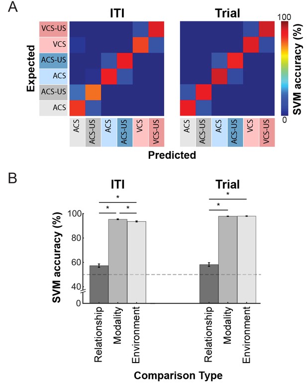
Ensemble firing patterns differentiated trial blocks more strongly depending on the CS modality and conditioning environment than CS-US relationship.
(A) Support Vector Machine (SVM) classifier was applied to binned firing rates during six trial blocks. Representative examples of confusion matrices indicating proportions of trial types that were identified by the SVM classifier correctly (warm colors along the diagonal) or misidentified as a different trial type (lighter colors off-diagonal). During CS-US pairings (trial) and inter-trial intervals (ITI), nearly all misclassifications were due to the confusion between CS-alone trials and CS-US paired trials. (B) Classification accuracy (mean ± SEM, 20 runs with 200 randomly subsampled cells) for binary discrimination along stimulus relationship (CS-alone vs. CS-US trials; Relationship), modality (auditory vs. visual CS trials; Modality), and conditioning environment (Box 1 vs. 2; Environment). In both task phases, the classification accuracy for Modality and Environment was higher than that for Relationship. *p<0.001 in posthoc Tukey HSD.
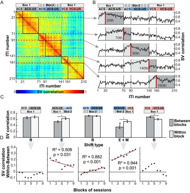
LEC ensemble activity showed an abrupt transition upon the shift of trial block involving changes in the conditioning environment and the stimulus modality.
(A) A matrix of state vector (SV) correlation in which the element rij represents the correlation coefficient between the SV computed during a 9 s interval (ITI) before the ith and jth CS presentation. The ITI number was continuously assigned to 210 ITIs according to the temporal order of six trial blocks as shown at the top of the matrix. The highlighted parts along the diagonal of the matrix (black squares) represent the r values between SVs within a trial block while the remaining parts represent those between different trial blocks. (B) The r for the last ITI in each trial block (red line) as a function of the temporal order of another ITI with which the r was computed. At the transition from the CS-alone block to the CS-US block in the same environment (20th, 90th, 160th), the r values with SVs in the same trial block (‘Within-block’, light-gray shading) was comparable to those with SVs in the following trial block (‘Between-blocks’, dark-gray shading). In contrast, the r value abruptly dropped upon the block shift including the change in the environment (70th) and CS modality (140th). (C) The Between-blocks r values (mean ± SD, n = 20 repeats with 100 subsampled cells) was significantly lower than the Within-block r values for two block shifts involving the environmental changes (E, E+M; *p<0.001 posthoc Tukey HSD), but not in the three shifts involving the stimulus contingency change (R). The Between-block r values were lower for the shift involving the changes in the CS modality and environment (E+M) than that involving the environmental change alone (E; #, p<0.001). (D) Over nine blocks of five sessions, the degree of ensemble transition (Within-block r minus Between-block r) increased for the block shift including the environmental and modality change (E+M), but decreased for the block shift including the environmental change alone (E).
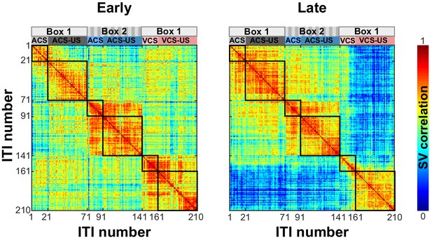
Changes in ensemble activity with experiences.
A matrix of state vector (SV) correlation during the first five sessions (Early) and the last five sessions (Late) as Figure 7A. Ensemble firing patterns differentiated trial blocks more strongly depending on the CS modality than conditioning environment only after repeated exposures to the fixed temporal structure of trial blocks.
Tables
Temporal order of the six trial blocks used for each rat.
| ID | 1ST | 2ND | 3RD | 4TH | 5TH | 6TH |
|---|---|---|---|---|---|---|
| RAT1 | ACS, Box 1 | ACS-US, Box 1 | ACS, Box 2 | ACS-US, Box 2 | VCS, Box 1 | VCS-US, Box 1 |
| RAT2 | ACS, Box 1 | ACS-US, Box 1 | ACS, Box 2 | ACS-US, Box 2 | VCS, Box 1 | VCS-US, Box 1 |
| RAT3 | ACS, Box 1 | ACS-US, Box 1 | ACS, Box 2 | ACS-US, Box 2 | VCS, Box 1 | VCS-US, Box 1 |
| RAT4 | VCS, Box 1 | VCS-US, Box 1 | ACS, Box 2 | ACS-US, Box 2 | ACS, Box 1 | ACS-US, Box 1 |
| RAT5 | ACS-US, Box 1 | ACS, Box 1 | ACS-US, Box 2 | ACS in Box 2 | VCS-US, Box 1 | VCS, Box 1 |
| RAT6 | ACS-US, Box 1 | ACS, Box 1 | ACS-US, Box 2 | ACS in Box 2 | VCS-US, Box 1 | VCS, Box 1 |
| RAT7 | ACS, Box 1 | ACS-US, Box 1 | ACS, Box 2 | ACS-US, Box 2 | VCS, Box 1 | VCS-US, Box 1 |
Number of recorded units and sessions in each rat.
| ID | Number of acquisition sessions | Number of sessions with recorded units | Total number of units |
|---|---|---|---|
| RAT 1 | 17 | 10 | 38 |
| RAT 2 | 16 | 12 | 61 |
| RAT 3 | 18 | 5 | 11 |
| RAT 4 | 16 | 13 | 49 |
| RAT 5 | 21 | 6 | 7 |
| RAT 6 | 20 | 13 | 55 |
| RAT 7 | 18 | 11 | 29 |
Number and percentage of cells with selective CS-evoked firing for three variables. Table summarizes the number of cells that significantly changed CS-evoked firing rates depending on CS-US relationship (CS-alone trials vs. CS-US paired trials, R), CS modality (auditory CS vs. visual CS, M), conditioning environment (Box 1 vs. Box 2, E), the combination of them, or none of them (Non-S). The values in parentheses show the percentage of cells in each category to total CS-responding cells.
| Site | Non-S | R | M | E | R+M | R+E | M+E | R+M+E |
|---|---|---|---|---|---|---|---|---|
| Overall 113 | 28 (24.8%) | 11 (9.7%) | 10 (8.8%) | 7 (6.2%) | 13 (11.5%) | 8 (7.1%) | 14 (12.4%) | 22 (19.5%) |
| Superficial layers 56 | 16 (28.6%) | 5 (8.9%) | 5 (8.9%) | 3 (5.4%) | 7 (12.5%) | 4 (7.1%) | 7 (12.5%) | 9 (16.1%) |
| Deep layers 57 | 12 (21.1%) | 6 (10.5%) | 5 (8.8%) | 4 (7.0%) | 6 (10.5%) | 4 (7.0%) | 7 (12.3%) | 13 (22.8%) |
Number and percentage of cells with selective firing for task variables during intervals between trials. Table summarizes the number of cells that showed selective firing rates for three task variables during intervals between trials, as shown in Table 3. The values in parentheses show the percentage of cells in each category to total non-responding, CS-responding, or all cells.
| Response type/Site | Non-S | R | M | E | R×M | R×E | M×E | R×M×E |
|---|---|---|---|---|---|---|---|---|
| Non-responding 137 | 3 (2.2%) | 11 (8.0%) | 5 (3.6%) | 1 (0.7%) | 30 (21.9%) | 20 (14.6%) | 12 (8.8%) | 55 (40.1%) |
| CS-responding 113 | 4 (3.5%) | 10 (8.8%) | 4 (3.5%) | 2 (1.8%) | 13 (11.5%) | 15 (13.3%) | 10 (8.8%) | 55 (48.7%) |
| Superficial layers 110 | 5 (4.5%) | 11 (10.0%) | 5 (4.5%) | 1 (0.9%) | 19 (17.3%) | 15 (13.6%) | 11 (10.0%) | 43 (39.1%) |
| Deep layers 140 | 2 (1.4%) | 10 (7.1%) | 4 (2.9%) | 2 (1.4%) | 24 (17.1%) | 20 (14.3%) | 11 (7.9%) | 67 (47.9%) |


