Research Article

Assessing the danger of self-sustained HIV epidemics in heterosexuals by population based phylogenetic cluster analysis

University Hospital Zurich, Switzerland
University of Zurich, Switzerland
Geneva University Hospitals, Switzerland
University Hospital Lausanne, Switzerland
University of Basel, Switzerland
University Hospital Basel, Switzerland
Regional Hospital Lugano, Switzerland
Lausanne University Hospital, Switzerland
Bern University Hospital, University of Bern, Switzerland
Cantonal Hospital St. Gallen, Switzerland

Sep 12, 2017

https://doi.org/10.7554/eLife.28721

Open access
Copyright information

Figures
Tables
Additional files

16 figures, 5 tables and 1 additional file

Figures

Figure 1

Download asset Open asset

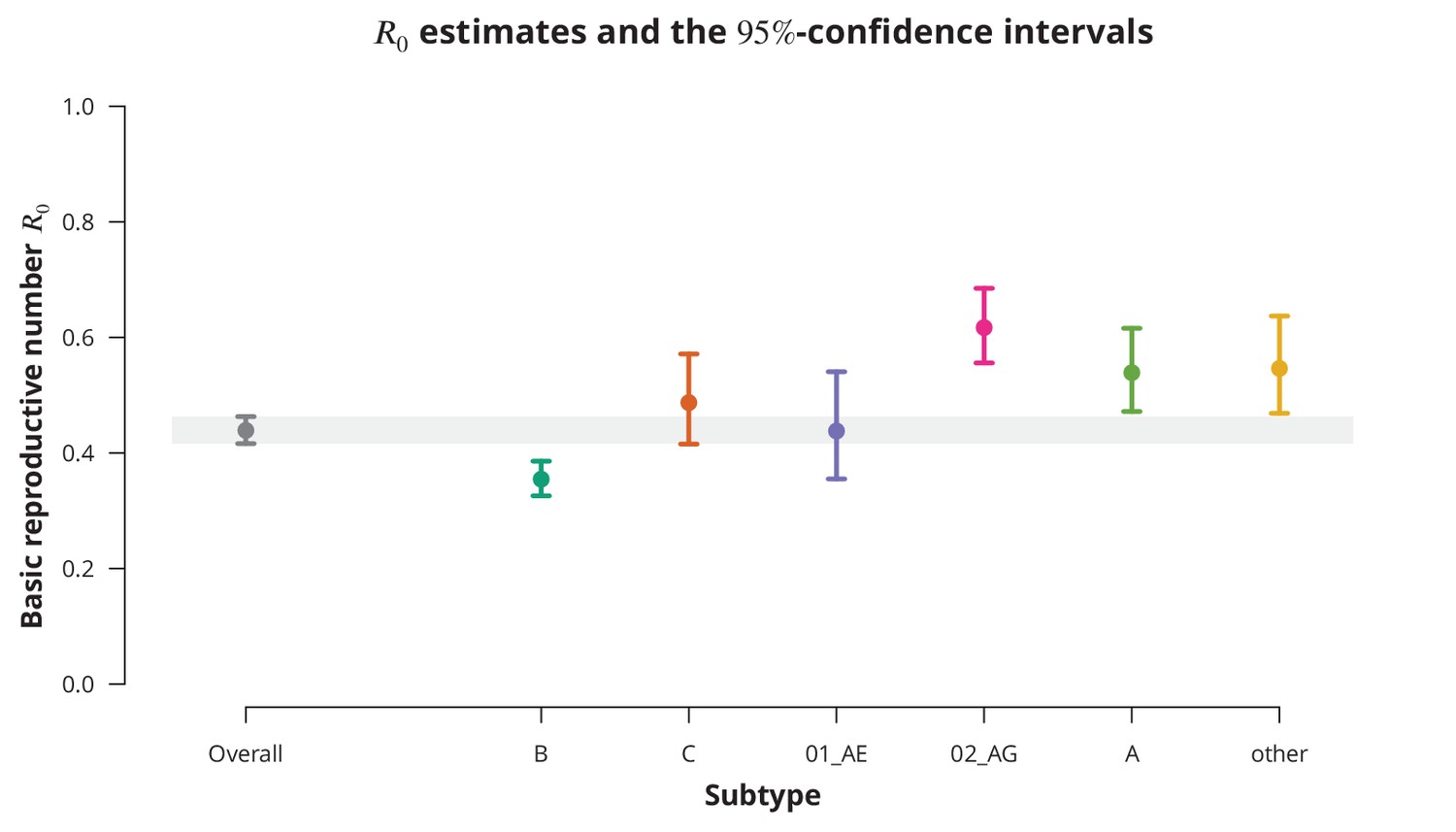
Overall basic reproductive number $R_{0}$ and $R_{0}$ per subtype from stratified analysis.

The dark gray point indicates the overall basic reproductive number $R_{0}$ estimate (by neglecting the transmission chain subtypes) and the corresponding $95 %$ -confidence interval is shown with the dark gray line and the gray-shaded band. The analogous results from the per-subtype stratified analysis are represented by colored points and lines, each color corresponding to one of the subtypes (B, C, CRF01_AE, CRF02_AG or A) or the group of subtypes (other).

https://doi.org/10.7554/eLife.28721.004

Figure 2

Download asset Open asset

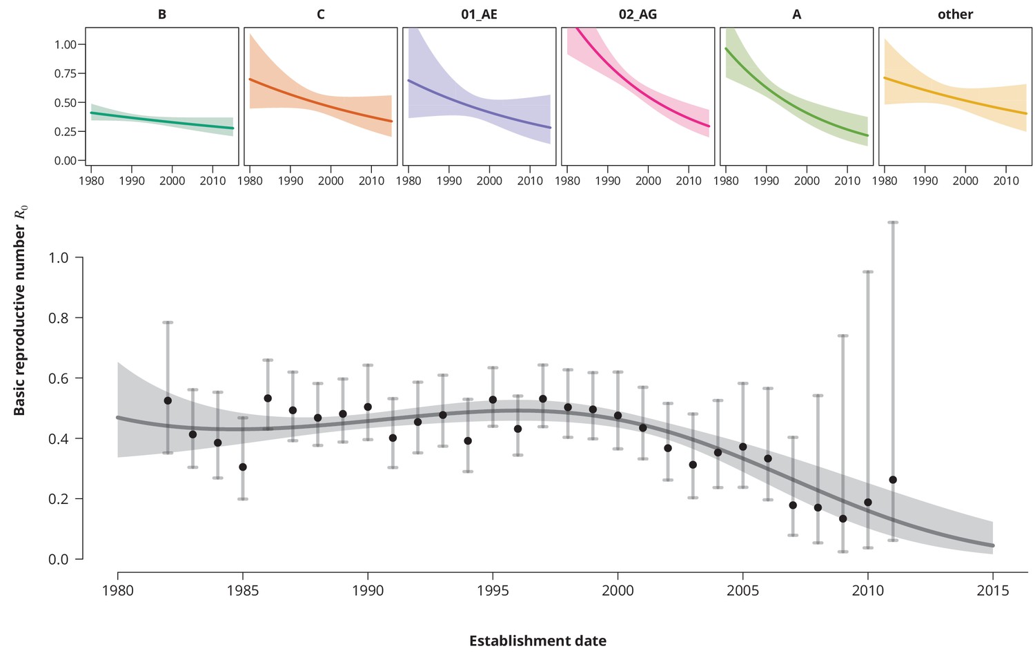
Time trends for $R_{0}$ .

The upper smaller panels show the time trends for $R_{0}$ from the subtype-stratified analyses, in which the $l o g (R_{0})$ ’s were modeled as linear functions of establishment date (i.e., for each subtype the time trend rate was assumed to be constant). The colored shaded-bands correspond to the $95 %$ -prediction bands. The (best-fitting) nonlinear time trend for $R_{0}$ from the overall analysis is displayed in the lower panel (dark gray curve) together with the $95 %$ -prediction band (gray-shaded area). The black points represent the $R_{0}$ estimates from the per establishment year stratified analyses and the gray vertical lines the corresponding $95 %$ -confidence intervals.

https://doi.org/10.7554/eLife.28721.005

Figure 3

Download asset Open asset

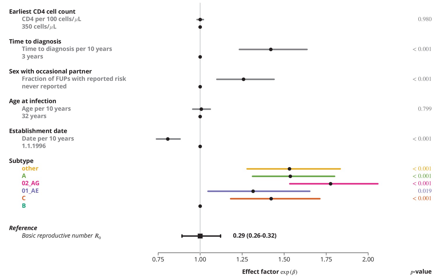
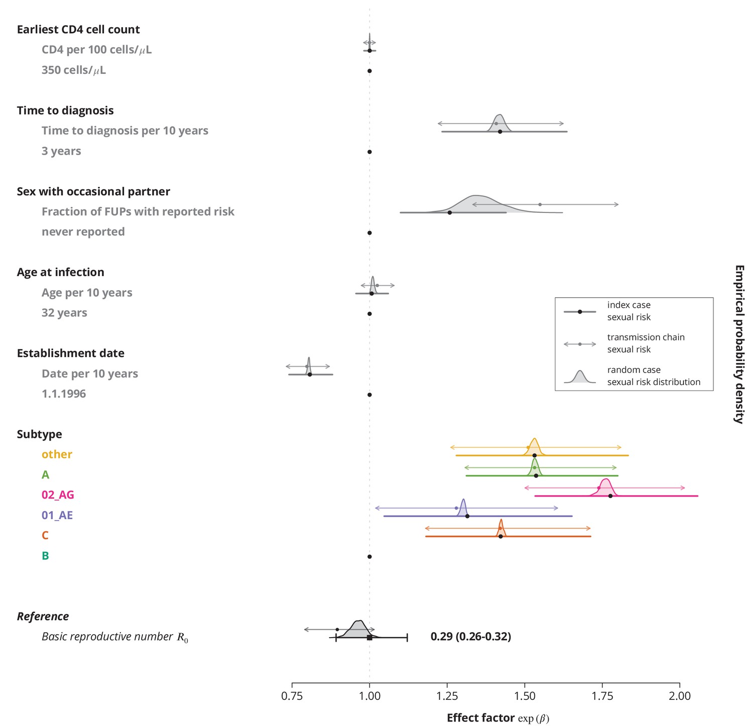
Effect of different factors on the basic reproductive number $R_{0}$ from the multivariate model with only linear factor terms.

The black square and the black line show the reference basic reproductive number $R_{0}$ and its $95 %$ -confidence interval (for a transmission chain of subtype B which started on 1.1.1996, and in which the index case was diagnosed 3 years after the infection, was 32 years old upon infection, never reported on having sex with occasional partner and had the earliest CD4 cell count of 350 cells per μL). The vertical gray line separates the factors associated with lower $R_{0}$ (left; effect factor $< 1$ ) and from the factors contributing to higher $R_{0}$ (right; effect factor $> 1$ ). The black points on this line refer to the reference transmission chain. The colored and dark gray lines represent the effect sizes from multivariate model (black circles depicting the estimates) for different factors and their $95 %$ -confidence intervals. The corresponding $p$ -values are shown in the rightmost column. FUP, follow-up visit.

https://doi.org/10.7554/eLife.28721.007

Figure 4

Download asset Open asset

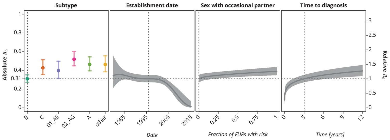
Final multivariate model’s profile plots of factors associated with the basic reproductive number $R_{0}$ .

The vertical dotted lines depict the reference transmission chain (of subtype B, started on 1.1.1996, in which the observed index case did not report having sex with occasional partner and was diagnosed after 3 years after the infection). The left $y$ -axis represents the basic reproductive number whereas the right $y$ -axis corresponds to the relative values of $R_{0}$ as compared to the baseline $R_{0}$ . The $R_{0}$ as the function of specific factor (with the other factors held fixed at the reference value) is displayed by the colored (for HIV-1 subtype) and the dark gray (establishment date, sexual risk behavior and time to diagnosis) lines. The vertical bars and the shaded bands, respectively, correspond to the $95 %$ -confidence intervals.

https://doi.org/10.7554/eLife.28721.008

Figure 5

Download asset Open asset

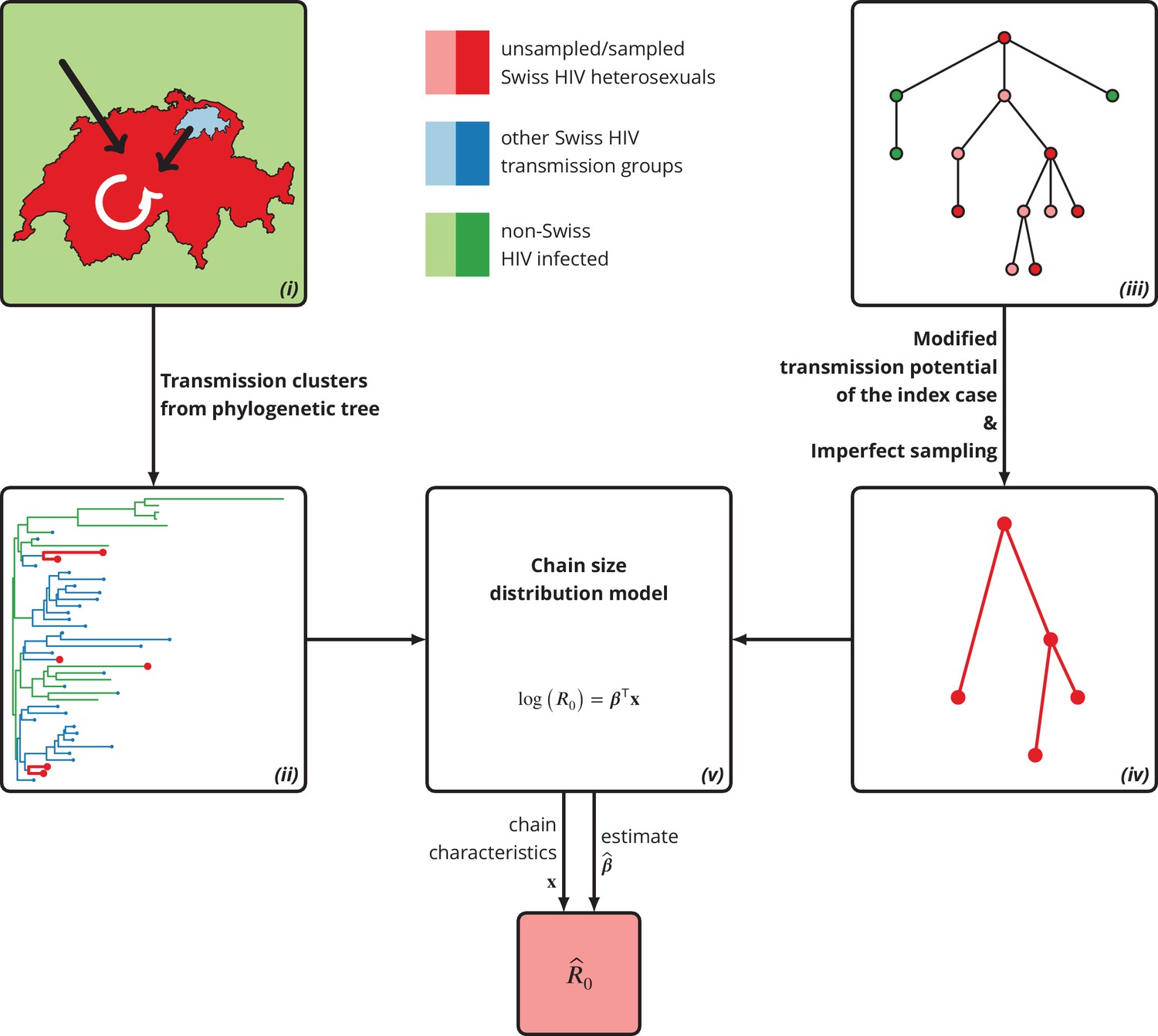
Graphical representation of our phylogeny-based statistical approach.

(i): HIV transmission among heterosexuals in Switzerland (white arrow) has never led to a self-sustained epidemic. However, the unknown potential of imported infections (black arrows) either from abroad or from other transmission groups in Switzerland remains a large concern. (ii): The HIV transmission chains corresponding to Swiss heterosexuals (depicted in red) were identified from the phylogenetic tree containing the SHCS and background viral sequences. (iii): Our mathematical model is based on the discrete-time branching process with nodes of three different types: sampled Swiss infection (red), unsampled Swiss infection (light red) and foreign infection infected by a Swiss index case before moving to Switzerland (green). (iv): Our method for inferring $R_{0}$ accounts for both imperfect sampling and modified transmission potential of the index case. (v): Moreover, it includes the baseline transmission chain characteristics to assess the determinants of $R_{0}$ .

https://doi.org/10.7554/eLife.28721.009

Appendix 1—figure 1

Download asset Open asset

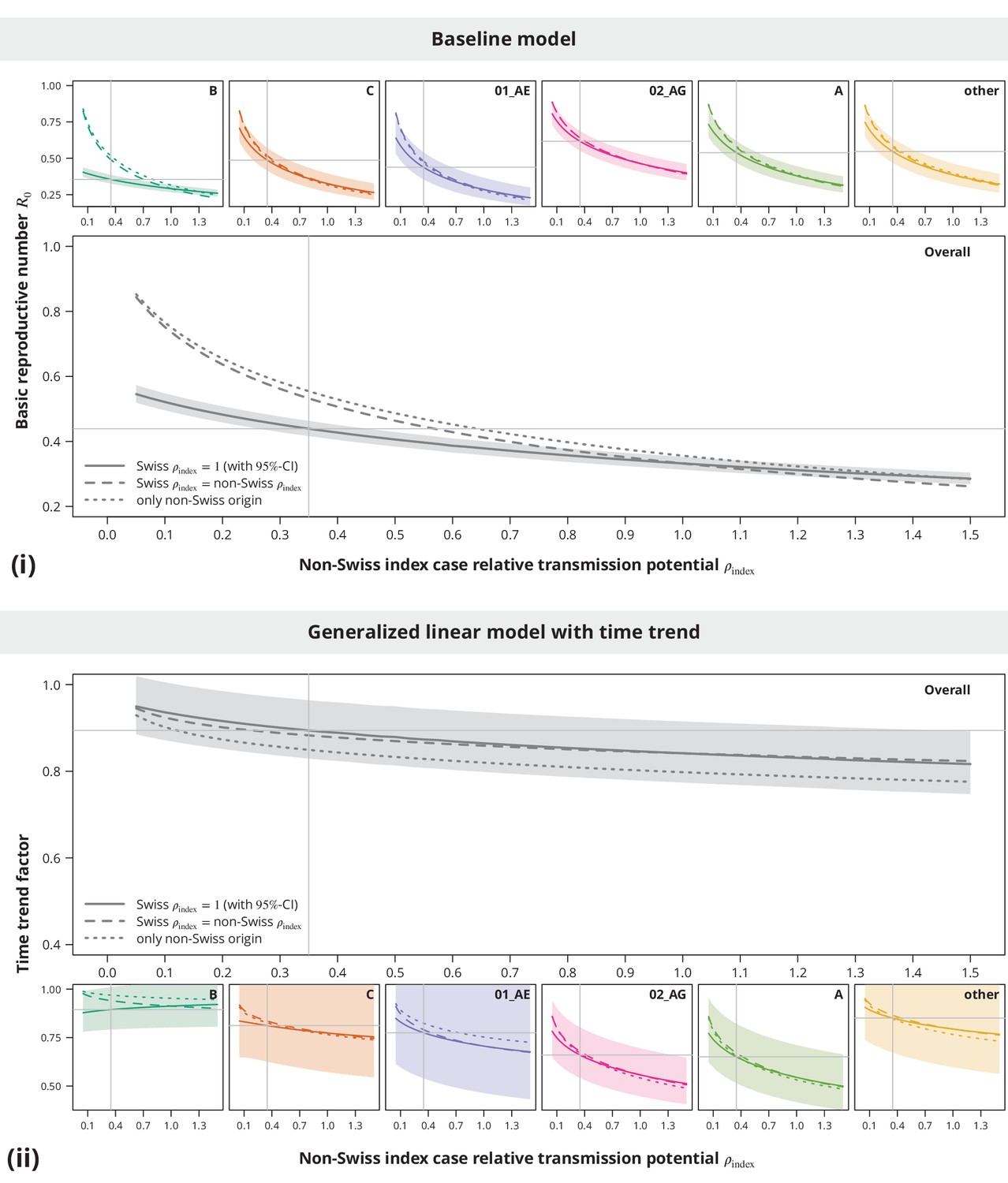
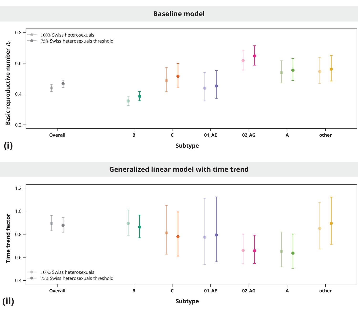
Sensitivity analysis regarding the index case relative transmission potential.

Panel (i) shows the sensitivity of the $R_{0}$ estimates from baseline model and panel (ii) the sensitivity of the time trend factor. The colored lines represent the subtype-stratified analyses, while the results from the overall models are shown in gray. In the first sensitivity analysis, the $ρ_{index}$ of Swiss-originating transmission chains was held at $1$ and the $ρ_{index}$ of non-Swiss origin varied (solid lines). In the second analysis, the $ρ_{index}$ of Swiss and non-Swiss origin was the same (dashed lines). The dotted lines show the results from the sensitivity subanalysis including only the transmission chains of non-Swiss origin. The vertical and horizontal lines depict the parameters and estimates from the main analysis, respectively.

https://doi.org/10.7554/eLife.28721.012

Appendix 1—figure 2

Download asset Open asset

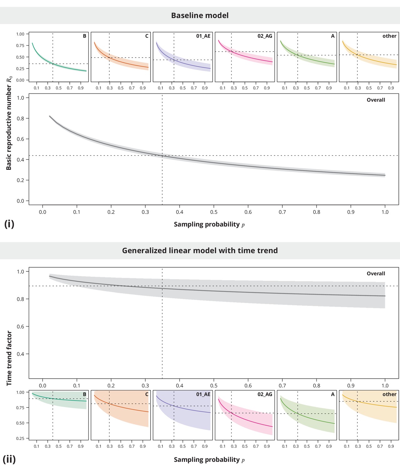
Sensitivity analysis regarding the sampling density.

The index case relative transmission potential parameter $ρ_{index}$ was the same as used in the main analyses, while the sampling densities varied ( $x$ -axis). In the pooled analysis (larger plots) the sampling density was the same for all transmission chains. Panel (i) shows the corresponding estimates of the basic reproductive number $R_{0}$ and the time trend factor estimates are displayed in panel (ii). The dotted vertical lines depict the sampling densities used for each subtype in our study (subtype-stratified plots) and the mean sampling density over all transmission chains (overall plots). The horizontal dotted lines represent the estimates from the main analysis.

https://doi.org/10.7554/eLife.28721.013

Appendix 1—figure 3

Download asset Open asset

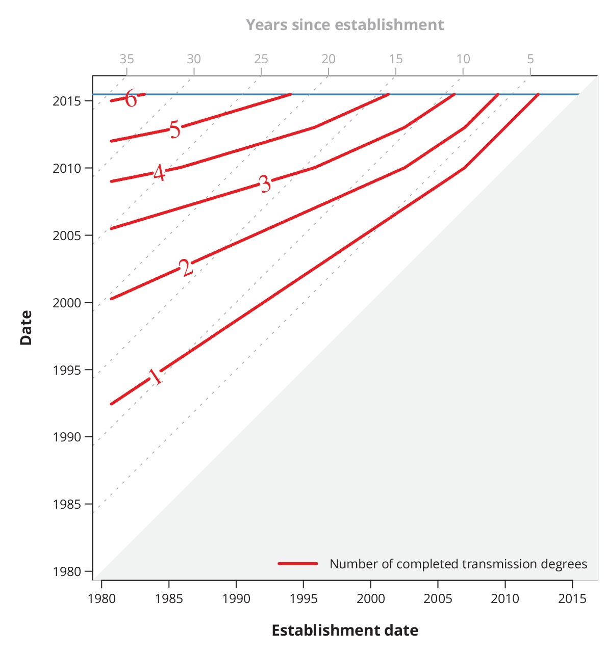
Conservative (with respect to ongoing transmission) maximum number of completed transmission degrees by a given date.

The red lines show the date ( $y$ -axis) by which at least a certain number (red numbers) of transmission degrees have been completed for a transmission chain with a specific establishment date ( $x$ -axis). The diagonal dotted gray lines depict the number of years since the establishment date, and the horizontal blue line represents the last sampling date.

https://doi.org/10.7554/eLife.28721.014

Appendix 1—figure 4

Download asset Open asset

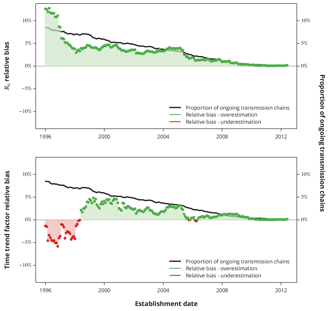
Relative bias due to ongoing transmission.

The upper panel shows the relative bias of the basic reproductive number $R_{0}$ from the baseline model and the lower panel the relative bias of the linear time trend factor from the corresponding generalized linear model. The proportion of active transmission chains over time is represented by the black line. The relative bias associated with overestimation and underestimation is displayed with green and red bars-points, respectively. Absence of bias is depicted by the horizontal gray lines.

https://doi.org/10.7554/eLife.28721.015

Appendix 1—figure 5

Download asset Open asset

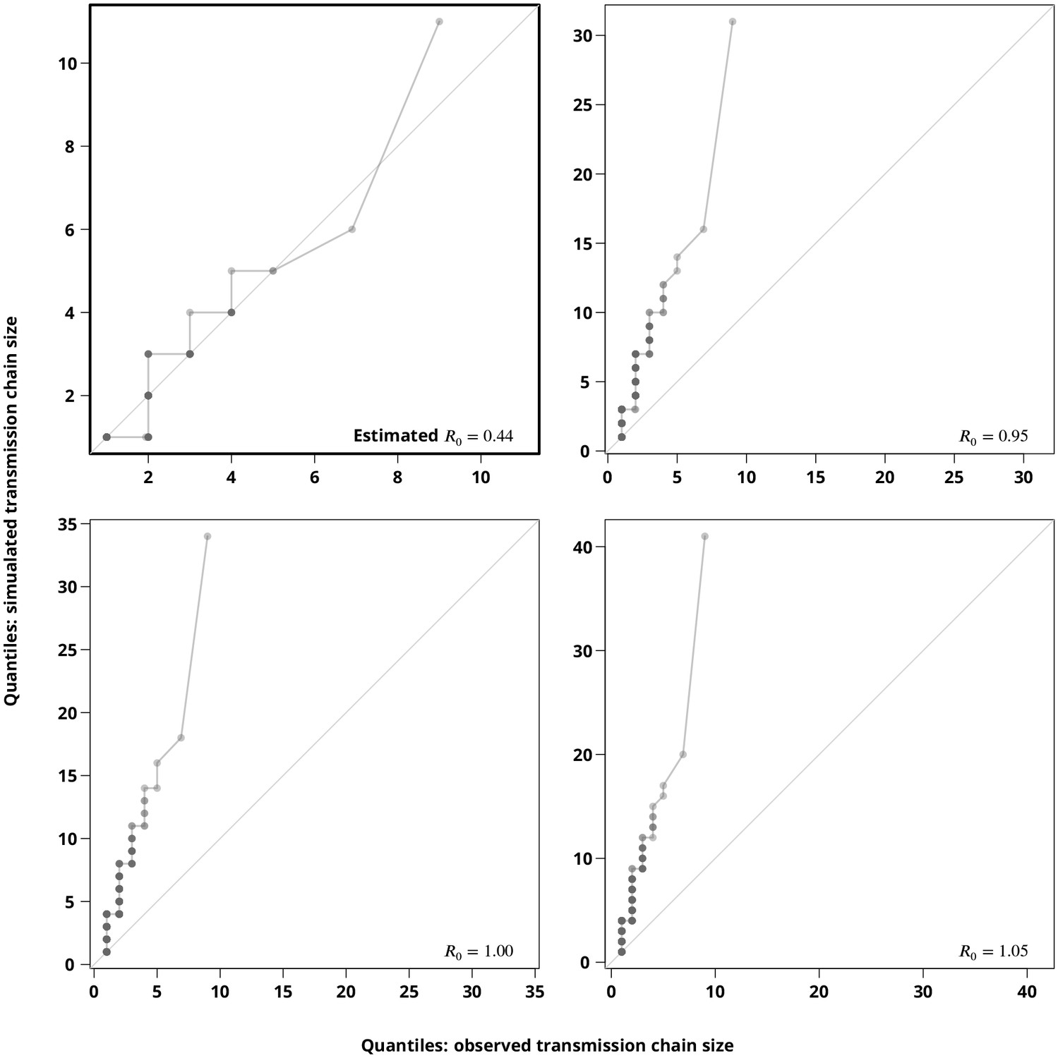
Sensitivity analysis regarding the stuttering transmission chains assumption.

The Q-Q plots compare the hypothetical transmission chain size distributions ( $y$ -axis showing their empirical permilles) with the transmission chain size distribution (empirical permilles on the $x$ -axis) inferred from the phylogeny. The upper left plot compares the distribution of the simulated transmission chain sizes based on the estimated $R_{0}$ with the (from the phylogeny) observed transmission chain sizes and thus verifies the $R_{0}$ estimate. The remaining plots compare the simulated transmission chain size distributions against the extracted transmission chain sizes for $R_{0}$ closer to $1$ to justify the subcritical transmission assumption. Each point represents a permille, hence the darker points indicate more overlapping permilles.

https://doi.org/10.7554/eLife.28721.016

Appendix 1—figure 6

Download asset Open asset

Comparison of effect sizes in the multivariate model with linear terms only for different sexual risk behavior definitions of a transmission chain.

The thick lines with black circles show the original effect sizes (where the index case determined the sexual risk behavior of the transmission chain) and their $95 %$ -confidence intervals. The empirical distribution of the effect sizes where a random individual in a transmission chain determines its sexual risk behavior is displayed by the shaded areas. The thinner horizontal double sided arrows with the filled circles correspond to the effect sizes and their $95 %$ -confidence intervals for the transmission chain level fraction of follow-up visits (FUPs) with reported sex with occasional partner by any of the infected individuals from the transmission chain. The vertical dotted gray line depicts the reference $R_{0}$ from the original model, i.e., using the index case to define the sexual risk behavior.

https://doi.org/10.7554/eLife.28721.017

Appendix 1—figure 7

Download asset Open asset

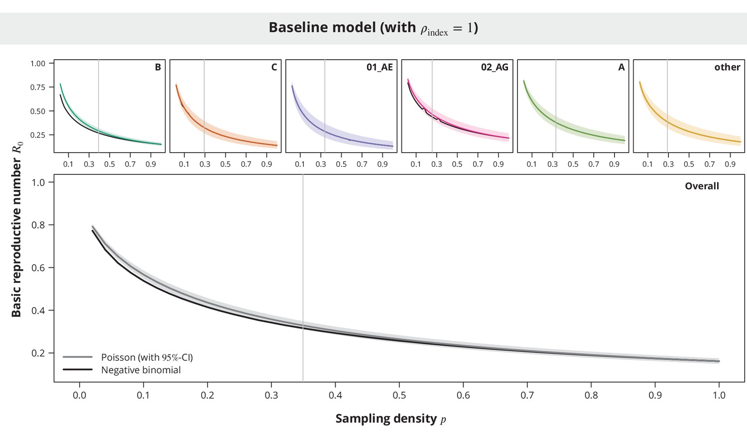
Comparison between the Poisson and the negative binomial offspring distribution baseline model $R_{0}$ estimates.

The dark gray and colored lines show the estimates from the model with Poisson offspring distribution, while the black lines correspond to the negative binomial distribution. The index case relative transmission potential parameter $ρ_{index}$ was fixed to $1$ and the sampling density ( $x$ -axis) varied. In the overall analysis the sampling density was the same for all transmission chains regardless of their subtype. The vertical gray lines depict the sampling densities used for each subtype in our study (above panels) and the mean sampling density in the overall analysis (bottom panel).

https://doi.org/10.7554/eLife.28721.018

Appendix 1—figure 8

Download asset Open asset

Sensitivity analysis regarding the transmission cluster definition.

The upper panel (i) compares the estimated $R_{0}$ with the original cluster definition (brighter lines) with the $R_{0}$ estimated based on the relaxed cluster definition (darker lines) from the overall analysis (in gray) and subtype-stratified analyses (in colors). Similarly, the bottom panel (ii) shows the comparison between the estimated time trend factors obtained from the transmission chain sizes based on different cluster definition thresholds.

https://doi.org/10.7554/eLife.28721.019

Appendix 1—figure 9

Download asset Open asset

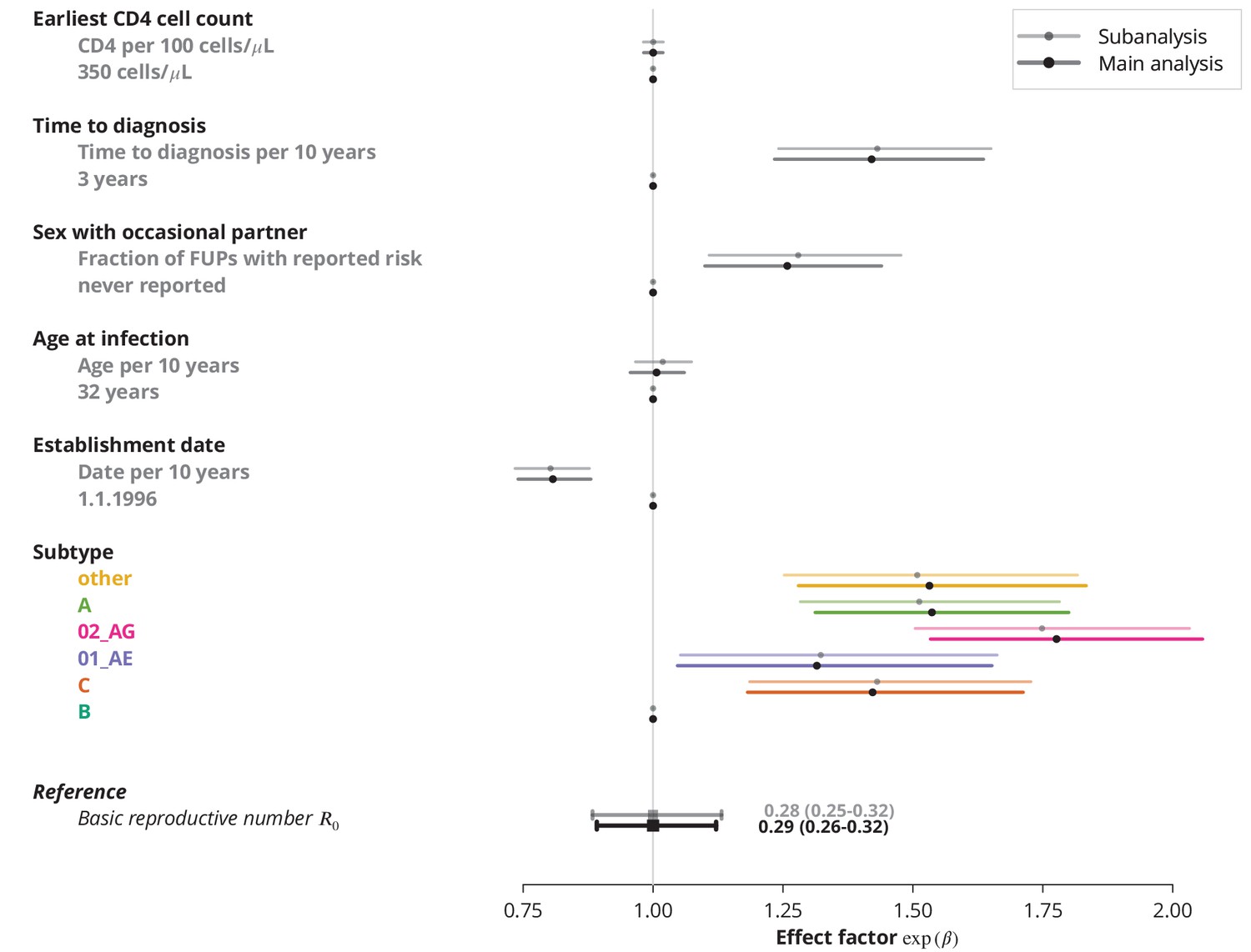
Subanalysis for the transmission chains with available follow-up information about sex with occasional partner of the index case compared to the main analysis with imputed data.

The effect sizes from the subanalysis are shown in brighter colors and those from the main analysis in dark. In the main analysis, the missing data were replaced by never reporting sex with an occasional partner.

https://doi.org/10.7554/eLife.28721.020

Appendix 1—figure 10

Download asset Open asset

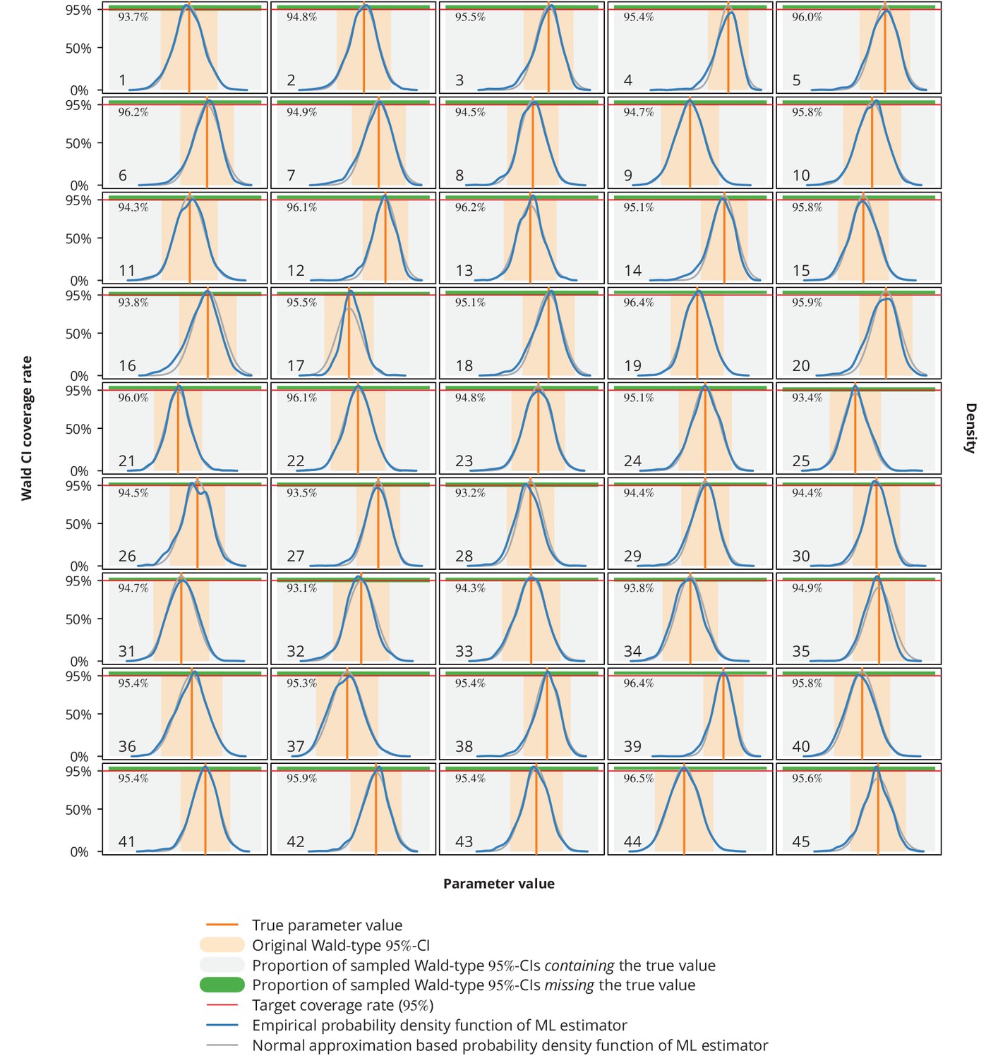
Empirical distribution of maximum likelihood (ML) estimator and the Wald-type confidence intervals (CI) coverage rates.

Each plot represents a single parameter from a single model (see Appendix 1—table 1 for the parameters overview including their values), where the number in the lower left corner denotes the parameter’s consecutive parameter number. The light gray-shaded area represents the proportion of the Wald-type $95 %$ -CIs from the parametric bootstrap simulations which contained the true value (depicted by the vertical orange line), while the green-shaded area corresponds to those CIs from the simulations that missed the true value. The numbers in the upper left corners are the coverage rates from the parametric bootstrap. The original Wald $95 %$ -CIs used in our study are displayed with the light orange-area. The dark blue and gray lines show the empirical distribution of ML estimators from the parametric bootstrap samples and the normal approximation based probability density function, respectively. The horizontal red lines depict the target coverage rate of $95 %$ .

https://doi.org/10.7554/eLife.28721.022

Appendix 1—figure 11

Download asset Open asset

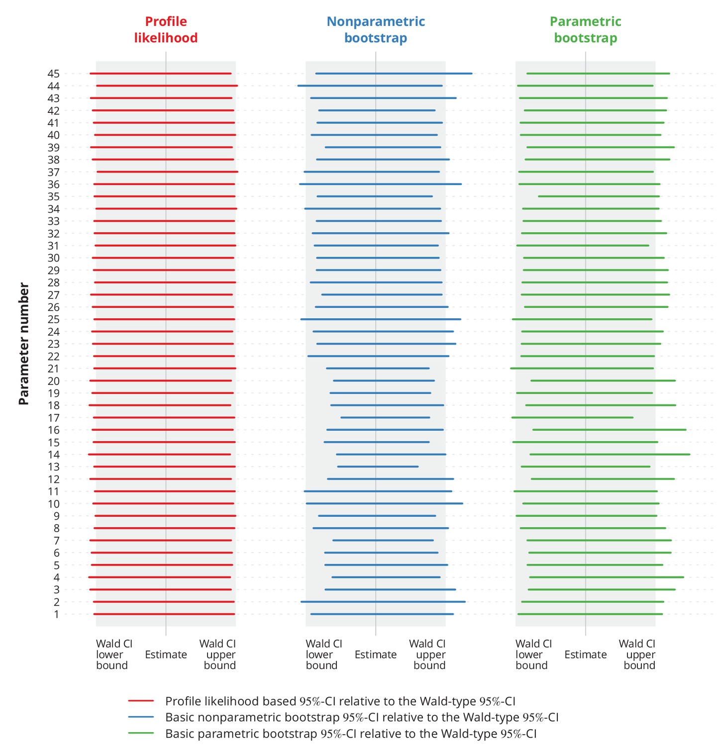
Comparison of different types of $95 %$ -confidence intervals (CI) with the normal approximation based Wald-type $95 %$ -CIs.

Each column corresponds to a different type of CIs, namely the profile likelihood based CIs, the basic nonparametric bootstrap CIs and the basic parametric bootstrap CIs. Each row represents a single parameter (the overview of the parameters is provided in Appendix 1—table 1). The colorful lines show the specific CIs compared to the corresponding Wald-type CIs, namely their relative widths and positions. The gray-shaded areas represent the Wald-type $95 %$ -CIs.

https://doi.org/10.7554/eLife.28721.023

Tables

Table 1

Transmission chain size distribution and model parameters.

https://doi.org/10.7554/eLife.28721.003

	Subtype						Overall
	B	C	01_AE	02_AG	A	Other	Overall
Total number of chains, $n$ (%)	1643 (53%)	322 (10%)	239 (7.7%)	331 (11%)	327 (11%)	238 (7.7%)	3100 (100%)
Chain size, $n$ (%)
1	1437 (87%)	280 (87%)	206 (86%)	272 (82%)	269 (82%)	195 (82%)	2659 (86%)
2	158 (9.6%)	34 (11%)	31 (13%)	40 (12%)	44 (13%)	36 (15%)	343 (11%)
3	30 (1.8%)	7 (2.2%)	1 (0.42%)	10 (3.0%)	10 (3.1%)	6 (2.5%)	64 (2.1%)
4	12 (0.73%)	-	1 (0.42%)	6 (1.8%)	3 (0.92%)	1 (0.42%)	23 (0.74%)
5	1 (0.06%)	1 (0.31%)	-	2 (0.6%)	1 (0.31%)	-	5 (0.16%)
6	1 (0.06%)	-	-	1 (0.3%)	-	-	2 (0.06%)
7	1 (0.06%)	-	-	-	-	-	1 (0.03%)
8	2 (0.12%)	-	-	-	-	-	2 (0.06%)
9	1 (0.06%)	-	-	-	-	-	1 (0.03%)
Sampling probability, $p$ (SD)	0.39	0.29	0.34	0.26	0.33	0.29	0.35 (0.05)
Chain origin, $n$ (%)
Swiss ( $ρ_{index} = 1$ )	948 (58%)	36 (11%)	36 (15%)	36 (11%)	47 (14%)	30 (13%)	1133 (37%)
non-Swiss ( $ρ_{index} = 0.35$ )	695 (42%)	286 (89%)	203 (85%)	295 (89%)	280 (86%)	208 (87%)	1967 (63%)

Table 2

Patients’ demographic characteristics.

https://doi.org/10.7554/eLife.28721.006

	Patients	Transmission chains
	Patients	Index case
Total number, $n$	3698	3100
Age at estimated date of infection [in years], median (IQR)	29.2 (23.1—37.8)	28.8 (22.8—37.4)
Estimated date of infection, median (IQR)	Jun 1996 (Sep 1990—Nov 2001)	Nov 1995 (Sep 1989—May 2001)
Time to diagnosis [in years], median (IQR)	3.40 (1.66—5.24)	3.54 (1.78—5.43)
Reported sex with occasional partner [as fraction of FUPs*], median (IQR)	0.53 (0.09—0.89)	0.50 (0.07—0.88)
No available FUP^†, $n$ (%)	250 (6.8%)	226 (7.3%)
Earliest CD4 count [per μL]^‡, median (IQR)	310 (143—510)	300 (134—507)

*Follow-up visit (FUP).

^†Patients without FUP questionnaire regarding the sexual risk behavior. See Sensitivity analyses.
^‡One patient did not have any available CD4 cell count. The missing value was imputed with the mean CD4 cell count.

Appendix 1—table 1

Overview of all the parameters, their estimates and the $95 %$ -confidence intervals fitted in all the models presented in this study.

https://doi.org/10.7554/eLife.28721.021

Subtypes	Parameter number	Parameter name	Parameter estimate	Wald-type $95 %$ -CI	Profile likelihood $95 %$ -CI
Overall	1	$\log (R_{0})$	$- 0.823$	$(- 0.876, - 0.770)$	$(- 0.878, - 0.772)$
B	2	$\log (R_{0})$	$- 1.037$	$(- 1.121, - 0.952)$	$(- 1.124, - 0.955)$
C	3	$\log (R_{0})$	$- 0.719$	$(- 0.879, - 0.559)$	$(- 0.892, - 0.571)$
01_AE	4	$\log (R_{0})$	$- 0.826$	$(- 1.036, - 0.615)$	$(- 1.057, - 0.632)$
02_AG	5	$\log (R_{0})$	$- 0.483$	$(- 0.587, - 0.378)$	$(- 0.594, - 0.384)$
A	6	$\log (R_{0})$	$- 0.618$	$(- 0.751, - 0.485)$	$(- 0.760, - 0.492)$
other	7	$\log (R_{0})$	$- 0.605$	$(- 0.758, - 0.451)$	$(- 0.771, - 0.461)$
Overall	8	$\log (R_{0, 𝑟𝑒𝑓})$	$- 0.839$	$(- 0.894, - 0.784)$	$(- 0.895, - 0.785)$
Overall	9	$\frac{{𝐷𝑎𝑡𝑒}_{𝑖𝑛𝑓𝑒𝑐𝑡𝑖𝑜𝑛} - 1.1.1996}{365 \cdot 10}$	$- 0.112$	$(- 0.187, - 0.037)$	$(- 0.188, - 0.037)$
B	10	$\log (R_{0, 𝑟𝑒𝑓})$	$- 1.070$	$(- 1.165, - 0.975)$	$(- 1.169, - 0.979)$
B	11	$\frac{{𝐷𝑎𝑡𝑒}_{𝑖𝑛𝑓𝑒𝑐𝑡𝑖𝑜𝑛} - 1.1.1996}{365 \cdot 10}$	$- 0.112$	$(- 0.234, 0.010)$	$(- 0.236, 0.008)$
C	12	$\log (R_{0, 𝑟𝑒𝑓})$	$- 0.692$	$(- 0.851, - 0.533)$	$(- 0.864, - 0.544)$
C	13	$\frac{{𝐷𝑎𝑡𝑒}_{𝑖𝑛𝑓𝑒𝑐𝑡𝑖𝑜𝑛} - 1.1.1996}{365 \cdot 10}$	$- 0.209$	$(- 0.466, 0.049)$	$(- 0.473, 0.046)$
01_AE	14	$\log (R_{0, 𝑟𝑒𝑓})$	$- 0.781$	$(- 0.991, - 0.570)$	$(- 1.013, - 0.588)$
01_AE	15	$\frac{{𝐷𝑎𝑡𝑒}_{𝑖𝑛𝑓𝑒𝑐𝑡𝑖𝑜𝑛} - 1.1.1996}{365 \cdot 10}$	$- 0.255$	$(- 0.616, 0.106)$	$(- 0.629, 0.101)$
02_AG	16	$\log (R_{0, 𝑟𝑒𝑓})$	$- 0.434$	$(- 0.539, - 0.329)$	$(- 0.545, - 0.333)$
02_AG	17	$\frac{{𝐷𝑎𝑡𝑒}_{𝑖𝑛𝑓𝑒𝑐𝑡𝑖𝑜𝑛} - 1.1.1996}{365 \cdot 10}$	$- 0.415$	$(- 0.609, - 0.222)$	$(- 0.615, - 0.226)$
A	18	$\log (R_{0, 𝑟𝑒𝑓})$	$- 0.725$	$(- 0.892, - 0.558)$	$(- 0.907, - 0.571)$
A	19	$\frac{{𝐷𝑎𝑡𝑒}_{𝑖𝑛𝑓𝑒𝑐𝑡𝑖𝑜𝑛} - 1.1.1996}{365 \cdot 10}$	$- 0.430$	$(- 0.660, - 0.199)$	$(- 0.672, - 0.209)$
other	20	$\log (R_{0, 𝑟𝑒𝑓})$	$- 0.600$	$(- 0.754, - 0.446)$	$(- 0.767, - 0.456)$
other	21	$\frac{{𝐷𝑎𝑡𝑒}_{𝑖𝑛𝑓𝑒𝑐𝑡𝑖𝑜𝑛} - 1.1.1996}{365 \cdot 10}$	$- 0.162$	$(- 0.397, 0.073)$	$(- 0.403, 0.072)$
Overall	22	$\log (R_{0, 𝑟𝑒𝑓})$	$- 0.710$	$(- 0.780, - 0.640)$	$(- 0.782, - 0.641)$
	23	${(\frac{{𝐷𝑎𝑡𝑒}_{𝑖𝑛𝑓𝑒𝑐𝑡𝑖𝑜𝑛} - 1.1.1996}{365 \cdot 10})}^{2}$	$- 0.313$	$(- 0.451, - 0.176)$	$(- 0.457, - 0.182)$
	24	${(\frac{{𝐷𝑎𝑡𝑒}_{𝑖𝑛𝑓𝑒𝑐𝑡𝑖𝑜𝑛} - 1.1.1996}{365 \cdot 10})}^{3}$	$- 0.184$	$(- 0.283, - 0.086)$	$(- 0.288, - 0.091)$
Overall	25	$\log (R_{0, 𝑟𝑒𝑓})$	$- 1.252$	$(- 1.366, - 1.137)$	$(- 1.369, - 1.140)$
	26	${𝑆𝑢𝑏𝑡𝑦𝑝𝑒}_{C}$	$0.352$	$(0.167, 0.538)$	$(0.158, 0.531)$
	27	${𝑆𝑢𝑏𝑡𝑦𝑝𝑒}_{01_𝐴𝐸}$	$0.274$	$(0.046, 0.502)$	$(0.029, 0.490)$
	28	${𝑆𝑢𝑏𝑡𝑦𝑝𝑒}_{02_𝐴𝐺}$	$0.575$	$(0.428, 0.721)$	$(0.426, 0.720)$
	29	${𝑆𝑢𝑏𝑡𝑦𝑝𝑒}_{A}$	$0.430$	$(0.271, 0.588)$	$(0.266, 0.584)$
	30	${𝑆𝑢𝑏𝑡𝑦𝑝𝑒}_{𝑜𝑡ℎ𝑒𝑟}$	$0.426$	$(0.247, 0.606)$	$(0.238, 0.600)$
	31	$\frac{{𝐷𝑎𝑡𝑒}_{𝑖𝑛𝑓𝑒𝑐𝑡𝑖𝑜𝑛} - 1.1.1996}{365 \cdot 10}$	$- 0.214$	$(- 0.301, - 0.127)$	$(- 0.301, - 0.128)$
	32	$\frac{𝐴𝑔𝑒 - 32}{10}$	$0.007$	$(- 0.045, 0.058)$	$(- 0.046, 0.057)$
	33	$\frac{CD4 - 350}{100}$	$0.000$	$(- 0.018, 0.019)$	$(- 0.019, 0.018)$
	34	${𝑅𝑎𝑡𝑒}_{𝑟𝑖𝑠𝑘}$	$0.230$	$(0.095, 0.364)$	$(0.096, 0.365)$
	35	$\frac{{𝑌𝑒𝑎𝑟𝑠}_{𝑑𝑖𝑎𝑔𝑛𝑜𝑠𝑖𝑠} - 3}{10}$	$0.351$	$(0.210, 0.492)$	$(0.207, 0.490)$
Overall	36	$\log (R_{0, 𝑟𝑒𝑓})$	$- 1.173$	$(- 1.301, - 1.045)$	$(- 1.304, - 1.048)$
	37	$\frac{1}{10} \log (\frac{{𝑌𝑒𝑎𝑟𝑠}_{𝑑𝑖𝑎𝑔𝑛𝑜𝑠𝑖𝑠}}{3})$	$1.727$	$(1.049, 2.405)$	$(1.064, 2.420)$
	38	${𝑆𝑢𝑏𝑡𝑦𝑝𝑒}_{C}$	$0.322$	$(0.140, 0.505)$	$(0.131, 0.498)$
	39	${𝑆𝑢𝑏𝑡𝑦𝑝𝑒}_{01_𝐴𝐸}$	$0.246$	$(0.020, 0.472)$	$(0.004, 0.460)$
	40	${𝑆𝑢𝑏𝑡𝑦𝑝𝑒}_{02_𝐴𝐺}$	$0.516$	$(0.374, 0.659)$	$(0.372, 0.658)$
	41	${𝑆𝑢𝑏𝑡𝑦𝑝𝑒}_{A}$	$0.404$	$(0.246, 0.562)$	$(0.241, 0.558)$
	42	${𝑆𝑢𝑏𝑡𝑦𝑝𝑒}_{𝑜𝑡ℎ𝑒𝑟}$	$0.401$	$(0.223, 0.580)$	$(0.214, 0.574)$
	43	${(\frac{{𝐷𝑎𝑡𝑒}_{𝑖𝑛𝑓𝑒𝑐𝑡𝑖𝑜𝑛} - 1.1.1996}{365 \cdot 10})}^{3}$	$- 0.231$	$(- 0.337, - 0.124)$	$(- 0.345, - 0.131)$
	44	$\sqrt{{𝑅𝑎𝑡𝑒}_{𝑟𝑖𝑠𝑘}}$	$0.230$	$(0.094, 0.366)$	$(0.096, 0.368)$
	45	${(\frac{{𝐷𝑎𝑡𝑒}_{𝑖𝑛𝑓𝑒𝑐𝑡𝑖𝑜𝑛} - 1.1.1996}{365 \cdot 10})}^{4}$	$- 0.129$	$(- 0.227, - 0.031)$	$(- 0.235, - 0.038)$

Appendix 2—table 1

Establishment date models obtained with the AIC/BIC forward selection and backward elimination and their respective AIC and BIC values as well as the $p$ -values from the likelihood ratio test compared to the null model without any covariates.

Terms that were part of the respective final model are marked by $\times$ .

https://doi.org/10.7554/eLife.28721.025

	AIC		BIC
	Forward	Backward	Forward	Backward
$\frac{{D a t e}_{i n f e c t i o n} - 1.1.1996}{365 \cdot 10}$
${(\frac{{D a t e}_{i n f e c t i o n} - 1.1.1996}{365 \cdot 10})}^{2}$		$\times$		$\times$
${(\frac{{D a t e}_{i n f e c t i o n} - 1.1.1996}{365 \cdot 10})}^{3}$	$\times$	$\times$	$\times$	$\times$
${(\frac{{D a t e}_{i n f e c t i o n} - 1.1.1996}{365 \cdot 10})}^{4}$	$\times$		$\times$
AIC	$3364.3$	$3364.2$	$3364.3$	$3364.2$
BIC	$3382.4$	$3382.3$	$3382.4$	$3382.3$
$p$ -value from LR test	$< 0.0001$	$< 0.0001$	$< 0.0001$	$< 0.0001$

Appendix 2—table 2

Multivariate models obtained with the AIC/BIC forward selection and backward elimination algorithms.

The terms listed in the table are the terms identified from the single determinant model selections and the crosses indicate the terms entering the multivariate models. The null model from the likelihood ratio test refers to the baseline model without any covariates (not even the subtype).

https://doi.org/10.7554/eLife.28721.026

	AIC		BIC
	Forward	Backward	Forward	Backward
$S u b t y p e$	$\times$	$\times$	$\times$	$\times$
${(\frac{{D a t e}_{i n f e c t i o n} - 1.1.1996}{365 \cdot 10})}^{2}$
${(\frac{{D a t e}_{i n f e c t i o n} - 1.1.1996}{365 \cdot 10})}^{3}$	$\times$	$\times$	$\times$	$\times$
${(\frac{{D a t e}_{i n f e c t i o n} - 1.1.1996}{365 \cdot 10})}^{4}$	$\times$	$\times$	$\times$
${𝑅𝑎𝑡𝑒}_{𝑟𝑖𝑠𝑘}$	$\times$	$\times$	$\times$	$\times$
$\sqrt{{R a t e}_{r i s k}}$	$\times$	$\times$	$\times$
$\frac{1}{10} \log (\frac{{Y e a r s}_{d i a g n o s i s}}{3})$		$\times$		$\times$
$\frac{\sqrt{{Y e a r s}_{d i a g n o s i s}} - \sqrt{3}}{\sqrt{10}}$	$\times$		$\times$
$\frac{{Y e a r s}_{d i a g n o s i s} - 3}{10}$	$\times$	$\times$	$\times$
${(\frac{\sqrt{{Y e a r s}_{d i a g n o s i s}} - \sqrt{3}}{\sqrt{10}})}^{3}$		$\times$		$\times$
$\frac{\sqrt{C D 4} - \sqrt{350}}{10}$
${(\frac{A g e - 32}{10})}^{2}$
AIC	$3254$	$3252$	$3254$	$3262$
BIC	$3314$	$3331$	$3314$	$3316$
$p$ -value from LR test	$< 0.0001$	$< 0.0001$	$< 0.0001$	$< 0.0001$

Additional files

Transparent reporting form: https://doi.org/10.7554/eLife.28721.010
Download elife-28721-transrepform-v2.pdf

Download links

A two-part list of links to download the article, or parts of the article, in various formats.

Downloads (link to download the article as PDF)

Article PDF

Open citations (links to open the citations from this article in various online reference manager services)

Mendeley

Cite this article (links to download the citations from this article in formats compatible with various reference manager tools)

Teja Turk
Nadine Bachmann
Claus Kadelka
Jürg Böni
Sabine Yerly
Vincent Aubert
Thomas Klimkait
Manuel Battegay
Enos Bernasconi
Alexandra Calmy
Matthias Cavassini
Hansjakob Furrer
Matthias Hoffmann
Huldrych F Günthard
Roger D Kouyos
Swiss HIV Cohort Study

(2017)

Assessing the danger of self-sustained HIV epidemics in heterosexuals by population based phylogenetic cluster analysis

eLife 6:e28721.

https://doi.org/10.7554/eLife.28721

Share this article

Cite this article

Overall basic reproductive number R0 and R0 per subtype from stratified analysis.

Time trends for R0.

Effect of different factors on the basic reproductive number R0 from the multivariate model with only linear factor terms.

Final multivariate model’s profile plots of factors associated with the basic reproductive number R0.

Graphical representation of our phylogeny-based statistical approach.

Sensitivity analysis regarding the index case relative transmission potential.

Sensitivity analysis regarding the sampling density.

Conservative (with respect to ongoing transmission) maximum number of completed transmission degrees by a given date.

Relative bias due to ongoing transmission.

Sensitivity analysis regarding the stuttering transmission chains assumption.

Comparison of effect sizes in the multivariate model with linear terms only for different sexual risk behavior definitions of a transmission chain.

Comparison between the Poisson and the negative binomial offspring distribution baseline model R0 estimates.

Sensitivity analysis regarding the transmission cluster definition.

Subanalysis for the transmission chains with available follow-up information about sex with occasional partner of the index case compared to the main analysis with imputed data.

Empirical distribution of maximum likelihood (ML) estimator and the Wald-type confidence intervals (CI) coverage rates.

Comparison of different types of 95%-confidence intervals (CI) with the normal approximation based Wald-type 95%-CIs.

Transmission chain size distribution and model parameters.

Patients’ demographic characteristics.

Overview of all the parameters, their estimates and the 95%-confidence intervals fitted in all the models presented in this study.

Establishment date models obtained with the AIC/BIC forward selection and backward elimination and their respective AIC and BIC values as well as the p-values from the likelihood ratio test compared to the null model without any covariates.

Multivariate models obtained with the AIC/BIC forward selection and backward elimination algorithms.

Transparent reporting form

Downloads (link to download the article as PDF)

Open citations (links to open the citations from this article in various online reference manager services)

Cite this article (links to download the citations from this article in formats compatible with various reference manager tools)

Overall basic reproductive number $R_{0}$ and $R_{0}$ per subtype from stratified analysis.

Time trends for $R_{0}$ .

Effect of different factors on the basic reproductive number $R_{0}$ from the multivariate model with only linear factor terms.

Final multivariate model’s profile plots of factors associated with the basic reproductive number $R_{0}$ .

Comparison between the Poisson and the negative binomial offspring distribution baseline model $R_{0}$ estimates.

Comparison of different types of $95 %$ -confidence intervals (CI) with the normal approximation based Wald-type $95 %$ -CIs.

Overview of all the parameters, their estimates and the $95 %$ -confidence intervals fitted in all the models presented in this study.

Establishment date models obtained with the AIC/BIC forward selection and backward elimination and their respective AIC and BIC values as well as the $p$ -values from the likelihood ratio test compared to the null model without any covariates.