Frequency-dependent mobilization of heterogeneous pools of synaptic vesicles shapes presynaptic plasticity
- CNRS, Université de Strasbourg, France
- University of Leipzig, Germany
Figures
Figure 1 with 1 supplement
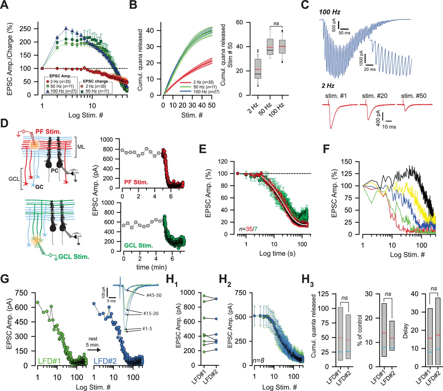
Low-frequency depression at GC-PC synapses.
(A) Averaged EPSC amplitude and charge versus stimulus number during train of stimuli at 2, 50 and 100 Hz. At 50 Hz EPSC amplitude and EPSC charge are represented by light and dark green squares, respectively. At 2 Hz, EPSC amplitudes and EPSC charge are represented with red diamonds and orange diamonds, respectively. Note strong facilitation at 50 and 100 Hz, no facilitation at 2 Hz. (B) Left and right panels represent the number of quanta released during trains of 50 stimuli at 2, 50 and 100 Hz. Left panel: Cumulative number of quanta release versus stimulus number at 2 Hz (red line), 50 Hz (green line) and 100 Hz (blue line). Note that the superposition of values at 50 Hz and 100 Hz mask the values at 100 Hz. Right panel: Box-plots showing the corresponding cumulative number of quanta released at the 50th stimulus. No difference was observed between 50 and 100 Hz (t-test, p=0.82). Mean and median values are indicated in red and black, respectively. (C) Representative recording traces of EPSCs evoked at 100 Hz and 2 Hz. Inset: The first EPSCs observed during 100 Hz train. The stimulus artifacts have been subtracted for the 100 Hz train. (D) left, schematics showing the two modes of stimulation. Extracellular stimulations in the molecular layer (ML) (upper panel) activated beams of PFs (in red) whereas stimulations of the granule cell layer (GCL) (lower panel) led to sparse activations of PFs (in green) Non-stimulated GCs are represented in light blue. Stimulated areas are represented by concentric orange circles. Right, two examples of the time course of EPSC amplitudes following stimulation of PFs (upper panel) or of GC somata (lower panel) at 0.033 Hz (gray points) and 2 Hz (red or green points respectively). (E) Mean normalized EPSC amplitude during sustained 2 Hz stimulations of PFs or GC somata (red and green points respectively). Note the delay before the actual induction of LFD. The depression was fitted by a monoexponential function (tau = 21.7 s, white line). (F) Selected time course of LFD recorded in 5 PCs showing differences in the onset and the plateau of depression. (G, H) LFDs elicited in the same cell share the same profile of depression. (G) Time courses of two successive LFDs elicited in the same cell. The second LFD protocol (LFD#2, blue points) was performed after a resting period of 5 min (LFD#1, green points). inset, traces correspond to averaged EPSCs recorded during LFD#1 and LFD#2 (green and blue traces, respectively) at the indicated stimulus numbers. (H1) EPSC amplitudes recorded at the first stimulus of LFD#1 (green points) and LFD#2 (blue points). The similar sizes of EPSC amplitudes in LFD#1 and LFD#2 indicates full recovery from depression during the resting period (paired t-test performed on EPSCs#1 of LFD#1 and LFD#2, p=0.94, n = 8). (H2) Superimposition of mean EPSC amplitudes recorded during LFD#1 (green points) and LFD#2 (blue points). Same set of experiment as in H1. (H3) Box-plots showing the cumulative number of quanta released during LFD#1 and LFD#2 (number of quanta released during LFD: 49.5 quanta ± 18.8 quanta for LFD#1 versus 45.6 quanta ±, 14.5 quanta for LFD#2, paired t-test, p=0.47, n = 8), the plateau of LFD#1 and LFD#2 (mean percentage of initial response for LFD: 13.9 ± 5.2% for LFD#1 versus 11.8% ±, 3.2 for LFD#2, paired t-test, p=0.39, n = 8) and the delay before the onset of depression (15.6 stimuli ± 6.6 stimuli for LFD#1 versus 17.4 stimuli ± 7.2 for LFD#2. paired t-test, p=0.13, n = 8). Since none of these parameters were statistically different between the two conditions, LFD#1 and LFD#2 were considered identical. Blue and red lines indicate median and mean values respectively. Same set of experiments as in H1, H2.
Figure 1—figure supplement 1
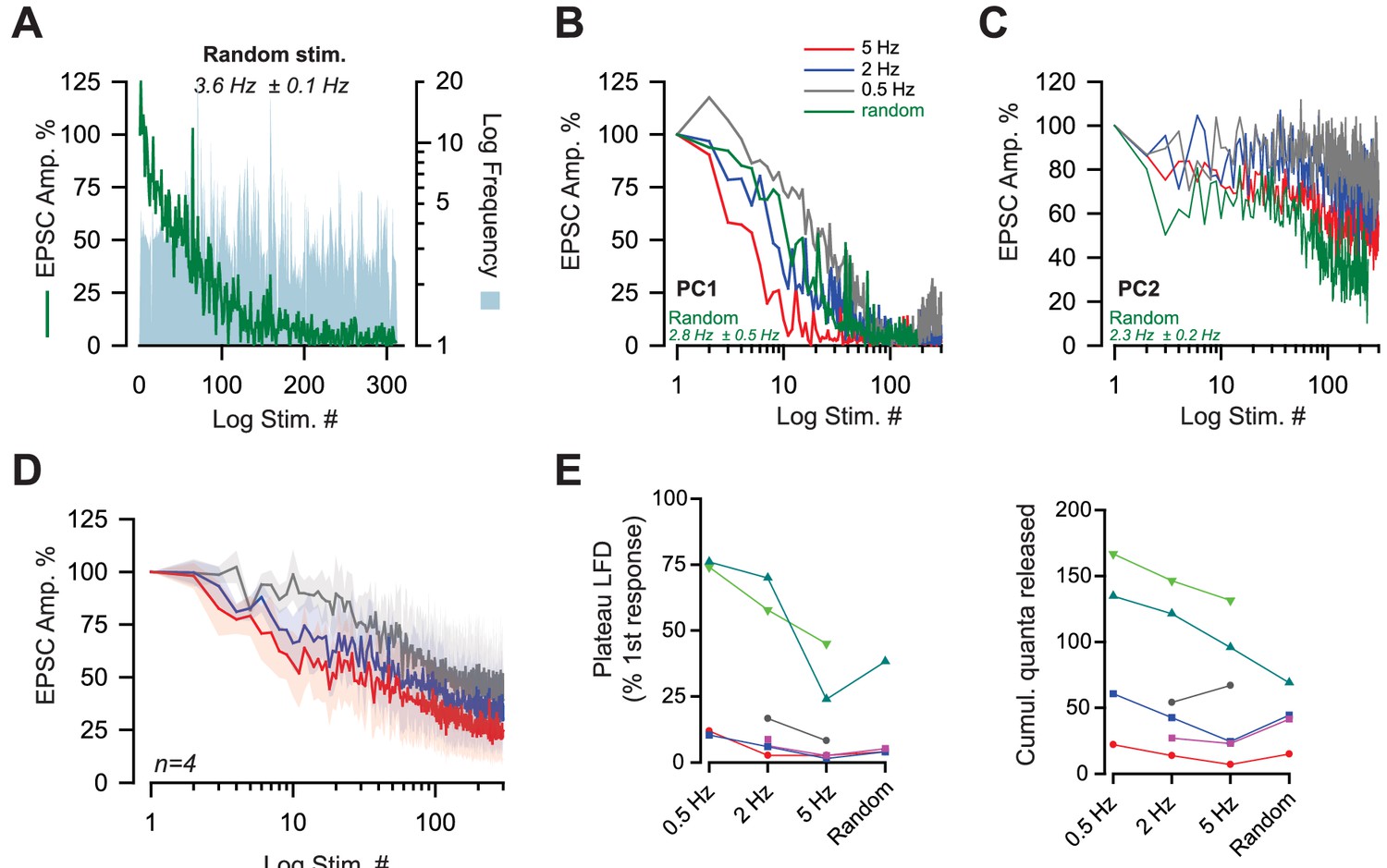
LFD can be elicited by a broad range of frequencies.
(A) Typical experiment illustrating EPSC amplitudes during LFD elicited by stimulations at random frequencies (frequencies ranging from 1 to 20 Hz) (green line). The instantaneous frequencies at any stimulus number are represented by the blue area. (B,C) Two examples of LFD elicited in two PCs (PC1 and PC2) using low frequencies at 0.5 Hz, 2 Hz, 5 Hz or random frequencies ranging from 0.5 Hz to 10 Hz (the value of the mean frequencies is indicated in green for each experiment). (D) Mean values of normalized EPSC during amplitudes plotted against stimulus number and recorded in PC after successive stimulation at 0.5, 2 and 5 Hz. (E) Values of the plateau of LFD (left graph) and of the cumulative number of quanta released obtained during LFD elicited with frequencies at 0.5 Hz, 2 Hz, 5 Hz or elicited with random frequencies. Each line corresponds to values obtained at the same PC.
Figure 2
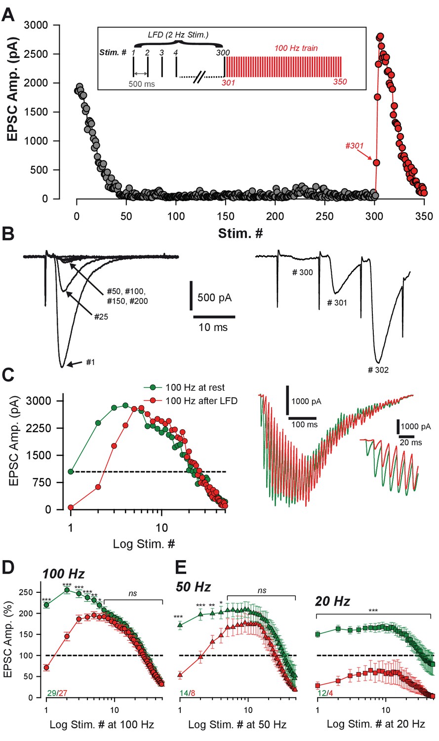
Ultrafast recovery from LFD by high-frequency trains.
(A) Typical experiment illustrating the time course of EPSC amplitude during LFD (gray points, stimulation at 2 Hz) and the fast recovery from LFD via high-frequency trains (red points, stimulation 100 Hz). Inset: protocol of stimulation. Stimulus #1 corresponds to the beginning of the 2 Hz stimulation. (B) Recording traces of superimposed EPSCs recorded during 2 Hz stimulation (left) and during the following 100 Hz train (right) at the indicated stimulus number from (A). Note the ultrafast recovery from depression at 100 Hz (stimulus # 301). (C) Left, Representative EPSC amplitudes evoked by a 100 Hz train applied before (green), and 10 ms after 300 stimuli at 2 Hz. The dashed line corresponds to the baseline amplitude defined as mean amplitude at 0.033 Hz. Note the similar size of EPSCs after the fourth stimulus at 100 Hz. Right, Corresponding traces recorded during these 100 Hz trains. Inset: The first EPSCs observed during train application. (D) Mean values of normalized EPSC amplitude elicited by trains of stimulation at 100 Hz at baseline (0.033 Hz, green) or after LFD induction (2 Hz, red). EPSC amplitudes were not significantly different after the seventh stimuli (MWRST, p=0.181, n = 27). (E) Mean values of normalized EPSC amplitude elicited by trains of stimulation at 50 Hz and 20 Hz at baseline (0.033 Hz, green) or after LFD induction (2 Hz, red). EPSC amplitudes were not significantly different after the after the fifth stimuli for 50 Hz trains (t-test, p=0.137, n = 13). EPSC amplitudes in 20 Hz trains elicited after LFDnever reached amplitudes of EPSCs of 20 Hz trains elicited at rest. Numbers at the bottom of the graphs indicate the number of cells recorded under each condition.
Figure 3

Short-term facilitation during triple-pulse stimulation at high frequency impedes recovery from LFD via high-frequency trains.
(A) Left panels an example of EPSC amplitudes during LFD followed by a 50 Hz train of stimulation. Right panel, upper trace, EPSCs elicited by the first stimulation at 2 Hz, middle traces, averaged EPSCs recorded during the LFD plateau (stimuli #280 to #300), bottom traces, EPSC recorded during the 50 Hz train applied 500 ms after the 2 Hz stimulation (artifacts subtracted). (B) left panels, time courses of EPSC amplitudes induced by triples pulse at different frequencies (LFDtriplet, see inset for protocol) as indicated and by a subsequent 50 Hz train. Right panel, upper trace, EPSCs elicited by the first triplet at 2 Hz, middle traces, averaged EPSCs recorded during the LFD plateau (stimuli #80 to #100), bottom traces, EPSC recorded during the 50 Hz train applied 500 ms after the 2 Hz stimulation (artifacts subtracted). For A and B, all data and traces were obtained in the same PC, and LFDs or LFDstriplet were elicited after a resting period of 5 min after the end of each protocol. (C) Mean values of normalized EPSC amplitudes evoked by 50 Hz train (left) and 100 Hz train (right) applied 500 ms after LFD induction (300 single stimuli at 2 Hz or 100 triple pulses at 2 Hz). Same color code than in A and B.
Figure 4 with 1 supplement
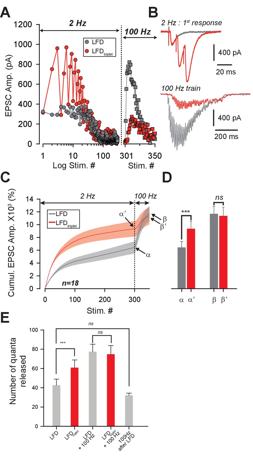
Recruitment of reluctant vesicles by high-frequency trains underpins recovery from LFD.
(A) Superimposition of ESPC amplitudes elicited during LFD (2 Hz, gray circles) or LFDtriplet (2 Hz with triplet stimulation at 100 Hz, red circles) in the same PC, and during the recovery from LFD via application of a 100 Hz train (gray squares for a 100 Hz train applied 500 ms after LFD, and red squares for a 100 Hz train applied 500 ms after LFDtriplet). (B) upper traces, superimposition of the first EPSCs recorded at stimulus #1 for LFD (gray trace) and LFDtriplet (red trace). Lower traces, EPSCs recorded during the 100 Hz trains applied 500 ms after LFD (gray trace) or 500 ms after LFDtriplet. (C) Mean values of cumulative EPSC amplitudes during LFD and LFDtriplet followed by a recovery train at 100 Hz (n = 18 cells). LFD and LFDtriplet were elicited successively in the same PCs. The dashed line indicates the beginning of the 100 Hz trains. α and α’ correspond to the cumulative value at the end of LFD protocols, β and β’ are values obtained following the recovery trains. (D) Mean values of a, a’, b andβ’ (same y axis as in C). (E) Estimation of the number of quanta released at GC-PC synapse during LFD, LFDtriplet and during the recovery via 100 Hz train (same set of experiments as in D). For the panels D and E, data were compared by using paired t-test.
Figure 4—figure supplement 1
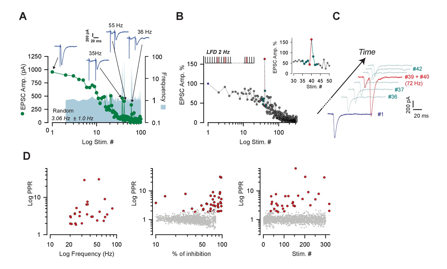
The status of the fully-releasable pool does not influence the mobilization of the reluctant pool.
(A) Typical experiment illustrating the time course of EPSC amplitudes during LFD elicited with random frequencies (frequencies ranging from 1 to 55 Hz, mean frequency indicated at the bottom of the graph) (green points). The instantaneous frequencies at any stimulus number are represented by the blue area. Traces illustrate strikingly high paired-pulse facilitation obtained when high frequencies were generated. (B) Extra stimuli applied randomly during the course of LFD elicited at 2 Hz. The paradigm of stimulation is illustrated on the top of the graph. Extra stimulations are shown as red bars and stimulation at 2 Hz are represented as black bars. The inset represent the same experiment with a focus on values of EPSC obtained just before and after an extra stimulus mimicking paired-pulse stimulation at 72 Hz. (C) EPSCs elicited at the indicated stimulus numbers in B. Blue, green and red traces correspond to the blue, green and red points in B. (D) The red points correspond to selected values of PPR obtained during paired-pulse stimulation at high frequencies elicited during the course of LFD at 2 or 5 Hz or during LFD elicited with random frequencies. These values correspond to strikingly high values of PPR, that is, with a Z-scorePPR >3.09. The Z-scorePPR at each stimulus number was calculated using the following equation: Z-scorePPR = (PPRstim# - PPRLFD)/(standard deviation PPRLFD) where PPRLFD corresponds to the mean value of PPR obtained at any stimulus number during the course of LFD at 2 Hz of 5 Hz. A Z-scorePPR >3.09 corresponds to a significance level <0.001. These values were plotted against the stimulus number (left graph), the percentage of inhibition (middle graph) or frequency of the paired-pulse stimulation (right graph). The gray points correspond to values of the PPR at 2 or 5 Hz obtained during LFD at 2 or 5 Hz.
Figure 5
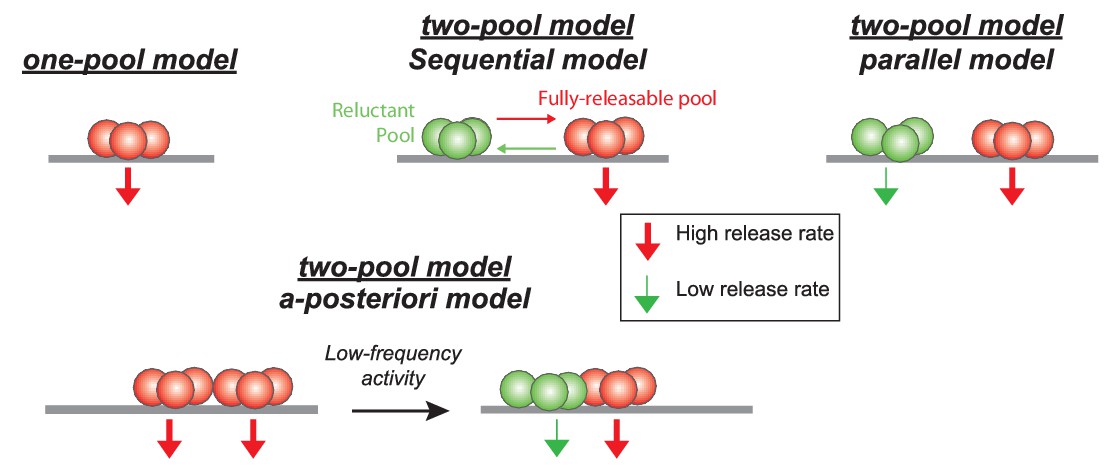
Schematics showing different models of SV release at GC-PC synapses.
Based on hypothesis proposed in other synapses, presynaptic release could be mediated by a homogeneous pool of release-ready SVs (one-pool model) or through a two-pool model with alternative stages of transition between the two pools. For the two-pool model, releasable SVs are separated in a fully-releasable pool (red SVs) or a reluctant one (green SVs).
Figure 6
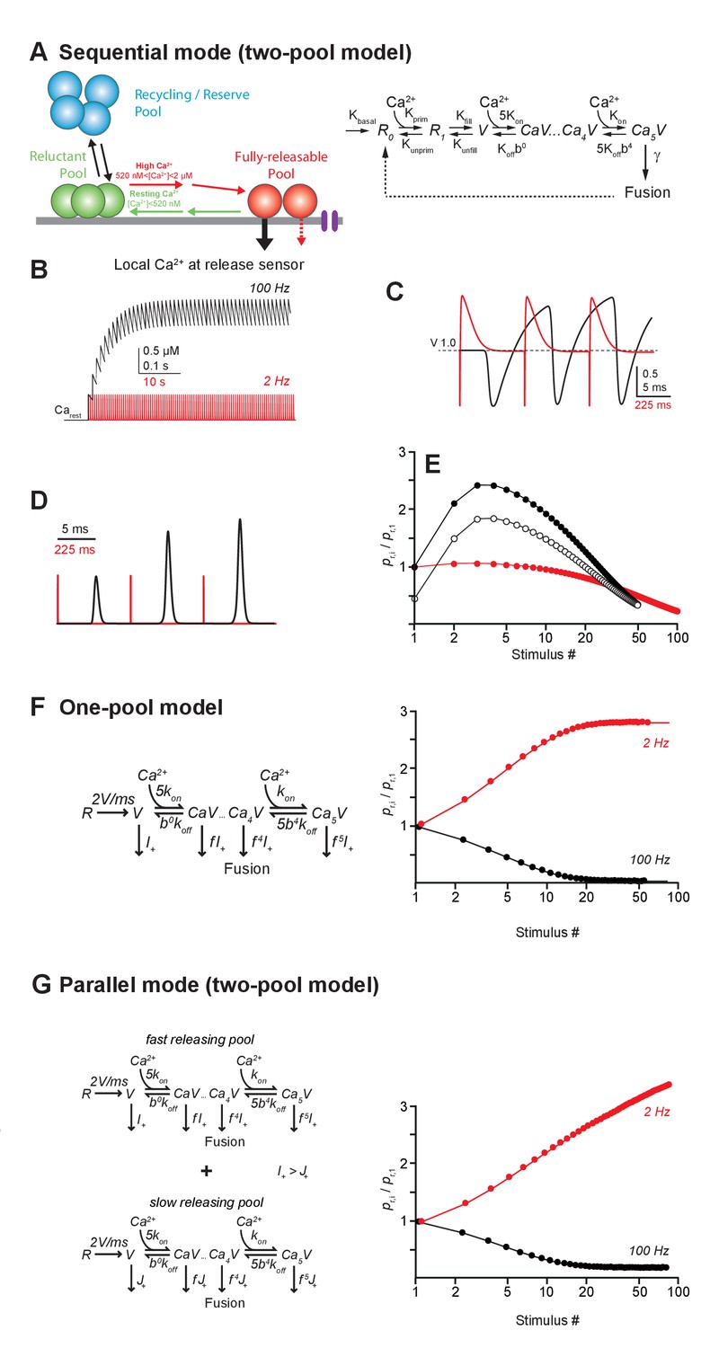
Models of LFD and short-term facilitation.
(A) Left, scheme illustrating the sequential model of Ca2+ binding and release at the PF-PC synapse. Voltage-dependent calcium channels are represented in purple.Right, in the corresponding mathematical model the recycling/reserve pool is contained only implicitly by restoration of the reluctant pool (R0+R1) from fused SVs (dashed arrow) and via a basal refilling rate (kbasal). Therefore, this model is referred to as sequential ‘two-pool’ model. During high-frequency stimulation, the residual Ca2+ increases, resulting in recruitment of SVs from the reluctant pool into the fully-releasable pool, that is, a temporal increase in the fully-releasable pool that enables short-term facilitation (red arrow). The residual Ca2+ generates an additional moderate, short-lasting facilitation due to slow unbinding from the release sensor (dashed red arrow). During low- frequency activation at 2 Hz, the residual Ca2+ drops back to resting level between stimuli and SVs recruited to the fully-releasable pool return to the reluctant pool (green arrow). (B) Simulated amplitudes of residual Ca2+ during high- (100 Hz, black) or low-frequency (2 Hz, red) activation starting from a resting Ca2+ (Carest) level of 50 nM. (C) Fraction of Ca2+ unoccupied SVs in the fully-releasable pool (V) of the release sensor during the initial three activations of a 100 Hz (black) or 2 Hz (red) activation train. Note that during the first three stimuli at low frequency, the fully-releasable pool relaxes to its initial (V = 1, i.e. 100%) from a transient overfilling (V > 1) prior to the next pulse. The fully-releasable pool continues to increase in size during high-frequency activation due to the build-up of residual Ca2+ and continuous recruitment of reluctant vesicles (cf. B). (D) Transmitter release rates during three stimuli at high (black) or low frequencies (red), normalized to the first release event (E) Paired-pulse ratios (PPRs) calculated as the ratio of release probabilities in the i-th (pr,i) and the first pulse (pr,1) during 100 Hz (filled black) or 2 Hz (red) stimulation. Open circles show PPRs during 100 Hz activations started in a previously depressed state. (F) Left, one-pool model of Ca2+ binding and release according to Wölfel et al., 2007 consisting of the ‘allosteric’ sensor model (Lou et al., 2005) supplemented with a reloading step of 2 SVs/ms. Right, in contrast to our experimental findings, this model generates low-frequency facilitation and high-frequency depression. (G) Left, as in F but for two parallel, non-interacting pools of SVs differing in their release rate constants thereby generating a ‘fast releasing pool of SVs’ (release rate I+ as in F) and a ‘slowly releasing pool of SVs’ (release rate J+<I+ as in F, Wölfel et al., 2007). Both models are restored via Ca2+ independent reloading steps of 2 SVs/ms. Right, note that similar to the model in F, this simulation generates a high-frequency depression and a low-frequency facilitation. Models in F and G fail to reproduce our experimental findings.
Figure 7
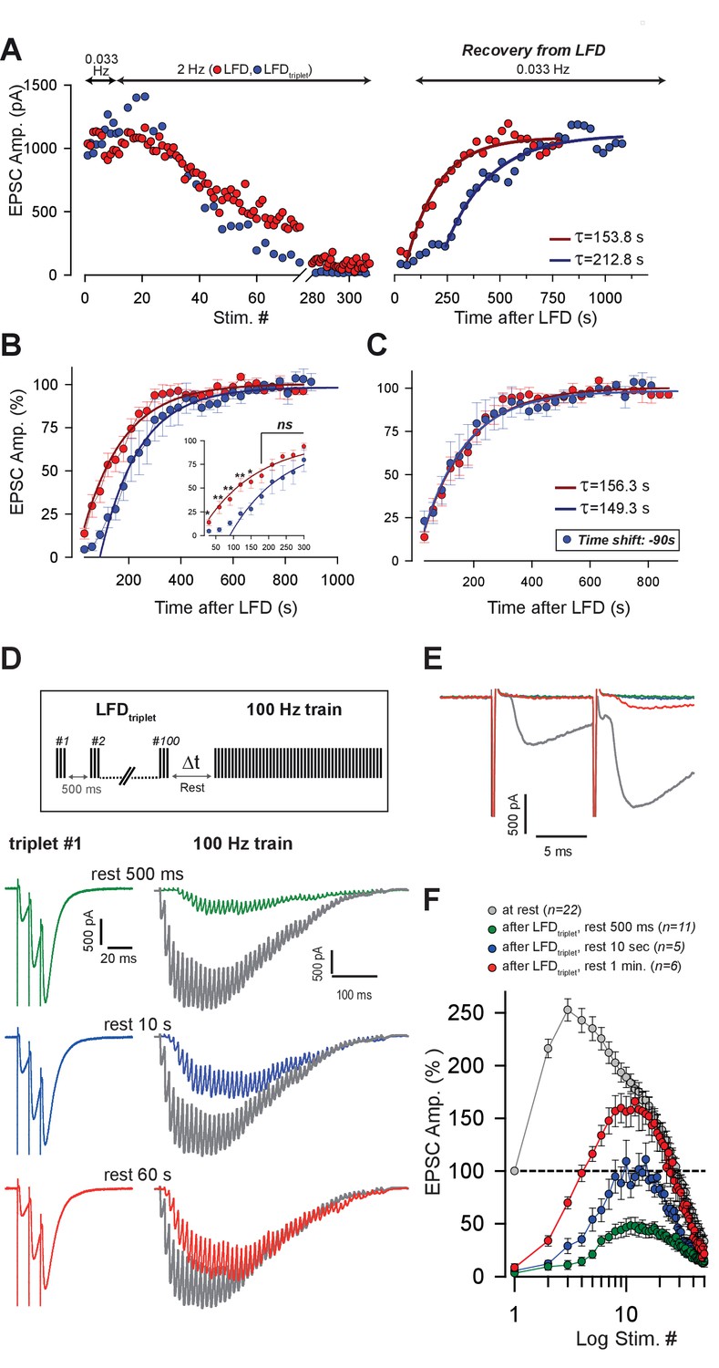
Kinetics of recovery from LFD and LFDtriplet.
(A) Left, superimposition of the time course of LFD and LFDtriplet (triplet stimulation at 200 Hz) elicited successively in the same cell after establishing a baseline of at least 10 successive stimuli at 0.033 Hz. Right, recovery from depression probed 30 s after the end of both LFD and LFDtriplet by a 0.033 Hz stimulation. For clarity, EPSC amplitudes were plotted against stimulus number in the left graph and against time in the right graph. The thick red and blue lines on the right graph show monoexponential fits. Note the delay of recovery after LFDtriplet, stimulation. (B) Normalized mean amplitudes of EPSCs evoked by 0.033 Hz stimulation 30 s after LFD (red points, n = 8) and after LFDtriplet (triplet stimulation at 200 Hz, blue points, n = 6). EPSC amplitudes were normalized to the mean value of EPSCs recorded during a baseline established by stimulation at 0.033 Hz. Thick red and blue lines represent monoexponential fits. (C) same values as in B, except that the time axis was shifted by 90 s for experimental values obtained during the recovery train applied after LFDtriplet (blue points). (D) Recovery from LFDtriplet probed by 100 Hz as indicated by the stimulation paradigm. Left, EPSC traces recorded during the 1st triplet stimulation at 2 Hz. Right, EPSC traces recorded during 100 Hz trains applied 500 ms, 10 s or 60 s after LFD protocol ended. Traces are superimposed with EPSCs recorded during a 100 Hz train applied before LFD induction (gray traces). (E) Superimposition of the first responses to the trains recorded in D. The color code is the same as in D. (F) Mean values of EPSC amplitudes recorded during 100 Hz trains applied 500 ms, 10 s or 60 s after the LFD protocol ended.
Figure 8
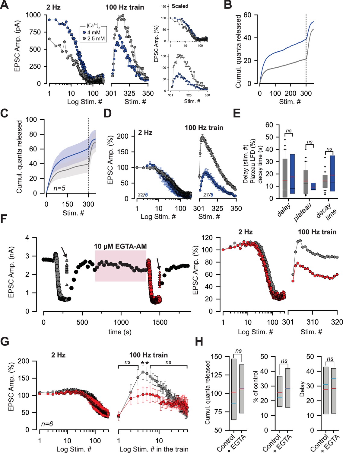
The reluctant pool can be recruited by increasing pr.
(A) Amplitude of ESPCs in the same PC during LFD (left panel) and during the recovery from LFD (middle panel) by a 100 Hz train before and after an increase in [Ca2+]e from 2.5 mM (gray points) to 4 mM (blue point). The right panels show the same experiment with EPSC amplitudes normalized with respect to the first response of LFD (B) Corresponding cumulative number of quanta release during LFD (stimuli #1 to #300) and during the recovery train (stimuli #301 to #350) in low and high [Ca2+]e. (same color code than in A). (C), Mean values of the cumulative number of quanta release during LFD (stimuli #1 to #300) and during recovery train at 100 Hz (stimuli #301 to #350) in low and high [Ca2+]e. The dashed line represents the end of the LFD protocol (same color code than in A). LFD and recovery trains were recorded in the same PCs. (D), Mean values of normalized EPSC amplitudes during LFD (left panel) and during the recovery via a 100 Hz train (right panel) in presence of 2.5 mM (gray points, same set of data than in Figure 1E for LFD and same set of data than in Figure 2D for recovery trains) and 4 mM [Ca2+]e (blue points). EPSC amplitudes were normalized with respect to the first response of LFD. (E) Box-plots showing the delay (mean number of stimuli before the onset of LFD: 14.5 ± 2.8, n = 30 at [Ca2+]e = 2.5 mM compared to 17.6 ± 8.0, n = 5, at [Ca2+]e=4 mM, MWRST, p=0.60), plateau of LFD (mean percentage of initial responses: 14.2 ± 2.0%, n = 30 at [Ca2+]e = 2.5 mM compared to 9.3 ± 1.4%, n = 5, at [Ca2+]e=4 mM, p=0.69, MWRST) and decay time (tau: 14.3 s ± 1.3 s, n = 30 at [Ca2+]e = 2.5 mM compared to 18.9 s ± 6.8 s, n = 5, at [Ca2+]e=4 mM, p=0.87, MWRST) in presence of 2.5 mM (gray boxes, same set of data than in Figure 1E for LFD and same set of data than in Figure 2D for recovery trains) and 4 mM [Ca2+]e (blue boxes). Black and red lines indicate median and mean values, respectively. (F) left, typical experiment showing the time course of EPSC amplitudes before and after application of 10 µM EGTA-AM. Black points correspond to EPSCs recorded during 0.033 Hz stimulation. Gray and red symbols correspond to EPSCs recorded during LFD (circles) and during the recovery trains at 100 Hz (triangles) before and after the bath application of 10 µM EGTA-AM respectively. Arrows indicate the application of a recovery train at 100 Hz. The pink box represents the bath application of 10 µM EGTA-AM. Right, corresponding ESPC amplitudes normalized with respect to the first response of LFD. (G) Mean EPSC amplitudes recorded during LFD (left panel) and during recovery trains (right panel) before (gray points) and after (red points) application of EGTA-AM. Note the difference in EPSC amplitudes evoked during the first stimuli at 100 Hz. Numbers at the bottom of the graphs indicate the number of cells recorded. (H) Box-plots showing the cumulative number of quanta released during LFD, the plateau of LFD and the delay before the onset of LFD before and after application of 10 µM EGTA-AM (same set of experiment as in G). None of these three parameters were statistically different between the two conditions (paired t-test, p=0.65, for the cumulative number of quanta released, paired t-test, p=0.39 for the plateau of LFD and paired t-test, p=0.89, for the delay, n = 6). Blue and red lines indicate median and mean values respectively.
Additional files
-
Transparent reporting form
- https://doi.org/10.7554/eLife.28935.012
Download links
A two-part list of links to download the article, or parts of the article, in various formats.
Downloads (link to download the article as PDF)
Open citations (links to open the citations from this article in various online reference manager services)
Cite this article (links to download the citations from this article in formats compatible with various reference manager tools)
Frequency-dependent mobilization of heterogeneous pools of synaptic vesicles shapes presynaptic plasticity
eLife 6:e28935.
https://doi.org/10.7554/eLife.28935


