Revealing the distribution of transmembrane currents along the dendritic tree of a neuron from extracellular recordings
- Hungarian Academy of Sciences, Hungary
- Pázmány Péter Catholic University, Hungary
- National Institute of Clinical Neurosciences, Hungary
- Neuromicrosystems Ltd., Hungary
- Nencki Institute of Experimental Biology of Polish Academy of Sciences, Poland
Figures
Figure 1
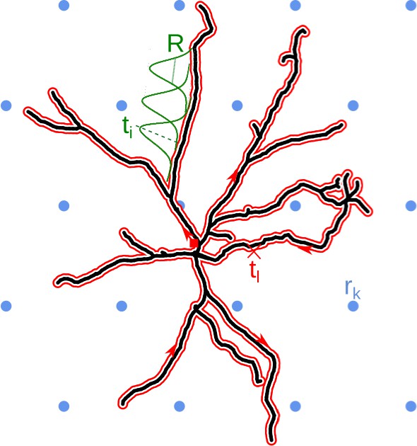
Schematic overview of the skCSD method.
The black line indicates the two-dimensional projection of the neuron on the MEA plane, the blue circles mark the location of multielectrode array (hexagonal grid, in this example), is the position of the electrode. The morphology in our method is described by a self-closing curve in three dimensions, which is indicated by red on the plot. We shall refer to this curve as the morphology loop. A point of the cell is visited once, if it is a terminal point of a dendrite, more than twice, if it is a branching point and twice in all the other cases. With this strategy, any point on the morphology loop uniquely identifies the physical location of the corresponding part of the cell unambiguously. To set up estimation framework, we distribute one-dimensional, overlapping Gaussian basis functions spanning the current sources. Several of these Gaussians are plotted in green, marks the center of the basis element, is the width parameter.
Figure 2
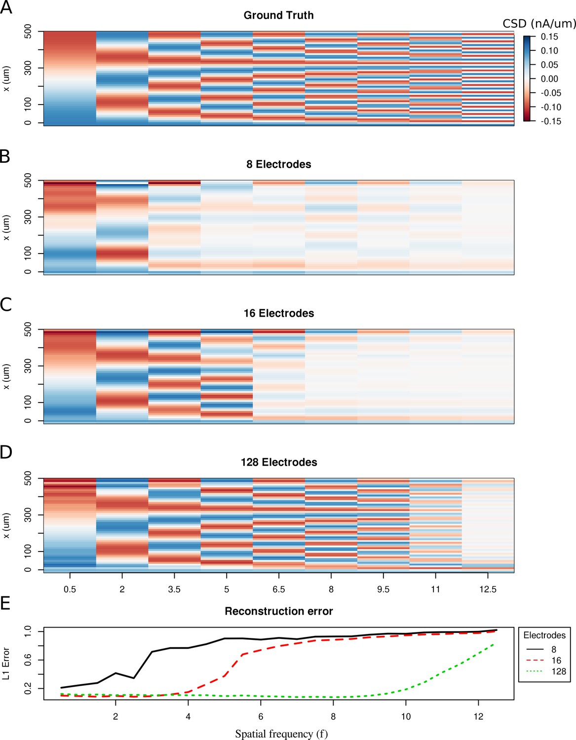
Limitations of the spatial resolution of the skCSD method in a simple ball-and-stick and laminar electrode setup.
(A) The ground truth membrane current source density distribution was constructed from cosine waves of increasing spatial frequency (x-axis) along the cell mophology (y-axis), which is shown in the interval representation. (B–D) skCSD reconstruction from 8, 16 and 128 electrodes. (E) The L1 Error of the skCSD reconstruction for 8 (black), 16 (red) and 128 (green) electrodes for CSD patterns of increasing frequency.
Figure 3
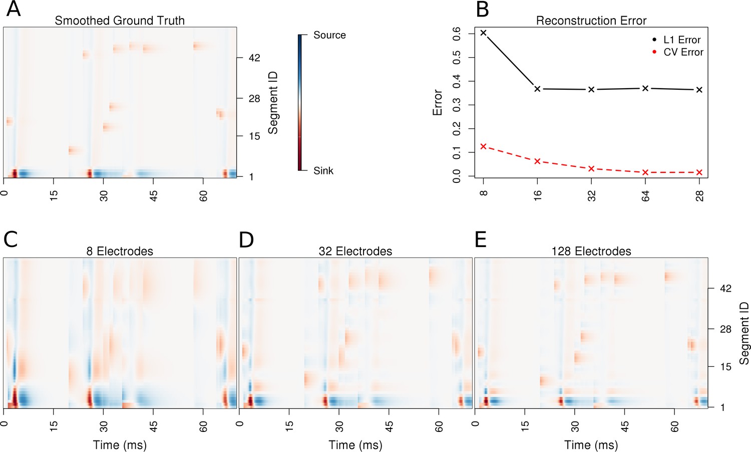
Performance of the skCSD method for a ball-and-stick neuron with random synaptic stimulation for recordings with a laminar probe placed 50 μm away from the cell.
(A) The ground truth spatio-temporal membrane current density in time (x-axis) along the cell in the interval representation (y-axis). The lowest segment is the soma, where the visible high amplitude of potential is a consequence of spiking. To make the much less pronounced synaptic activity on the dendritic part visible, nonlinear color map was used. Panel (B) shows the lowest values of cross-validation and L1 error for the before-mentioned setups. Panels (C–E) present the best skCSD reconstruction in case of recording with 8, 32, and 128 electrodes. One can see how increasing the number and density of probes in the region improves the reconstruction quality until a certain level. CV error was used here to select the parameters leading to the best reconstructions.
Figure 4
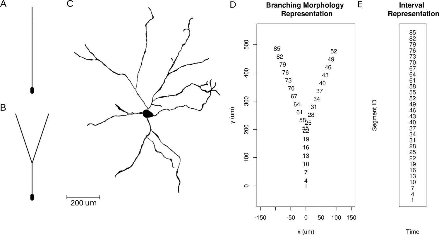
Neuron morphologies used for simulation of ground truth data.
(A) Ball-and-stick neuron. (B) Y-shaped neuron. (C) Ganglion cell.
Figure 5
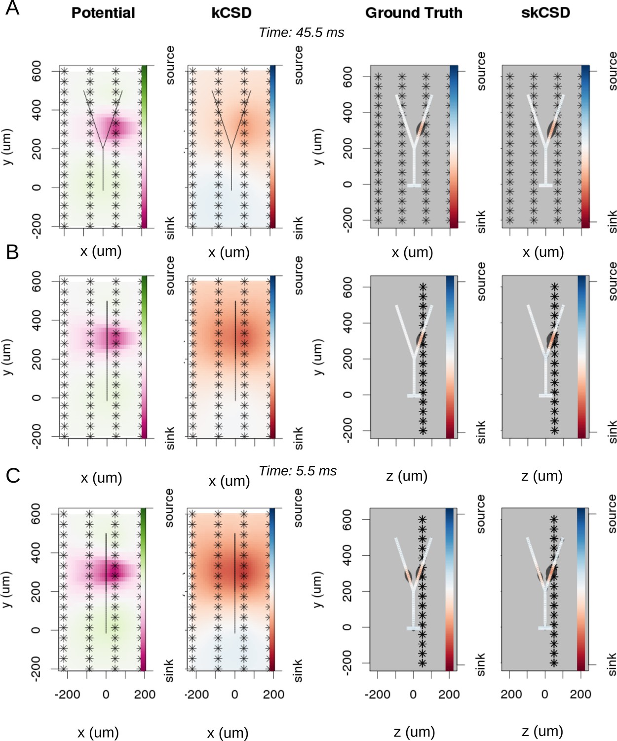
Reconstruction of synaptic inputs on a Y-shaped neuron with a regular rectangular 4 × 16 electrode grid.
Each panel (A–C) shows the spline-interpolated extracellular potential (V), followed by standard kCSD reconstruction, both at the plane of the 4 × 16 electrodes’ grid used for simulated measurement. Then, the ground truth and skCSD reconstruction are shown in the branching morphology representation in the plane containing the cell morphology. Each figure shows superimposed morphology of the cell. Note that in panel A the grid is parallel to the cell, while in panels (B–C) it is perpendicular. The dark gray shapes are guides for the eye and are sums of circles placed along the morphology with radius proportional to the amplitude of the sources at the center of the circle. (A) Shows results for a synaptic input depolarizing one branch. (B) Shows the same current distribution as in the previous setup, but the grid is rotated by 90 degrees. (C) A synaptic input is added to the other branch. Observe that in all three cases, the interpolated potential and the standard CSD reconstruction, which can be drawn only in the plane of the electrodes’ grid, do not differ significantly, hence they cannot distinguish between these three situations. On the other hand, skCSD method is able to identify correctly both synaptic inputs.
Figure 6
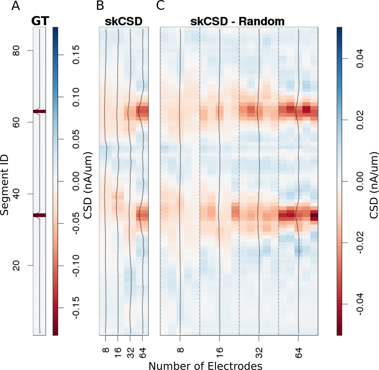
Reconstruction of synaptic inputs placed on different branches of the Y-shaped neuron for electrodes arranged regularly and randomly within the same area.
We use the interval representation for visualization. The numbers on horizontal axis enumerate different electrode setups. The black profiles show the averaged membrane current as reconstructed in a given case; for random electrode distribution these are averages over five different realizations. (A) Ground truth membrane currents, the strong red indicates the synaptic inputs. (B) Reconstruction results for 8 (4 × 2), 16 (4 × 4), 32 (4 × 8), and 64 (4 × 16) electrodes arranged regularly. The skCSD reconstruction improves with the number of electrodes as the color representation and the black profiles indicate. (C) When distributing the same numbers of electrodes on the same plane as in the previous case, the quality of the average skCSD reconstruction, as indicated by the black profiles, is similar.
Figure 7
The effects of basis properties on reconstruction quality.
We used the Y-shaped morphology and the 4 × 4 electrode setup to investigate the effect of using various basis numbers for the reconstruction. L1 error was calculated to compare the results for basis with elements, for several values of basis width and . With few basis sources one cannot recover CSD properly. As the number of basis functions increases, the reconstruction error is minimized for moderate values of and for narrow basis sources, which can best resolve small details of the CSD to be reconstructed.
Figure 8

skCSD reconstruction of dendritic backpropagation patterns for a retinal ganglion cell model driven with oscillatory current.
(A) Somatic membrane potential during the simulation. The red line marks the time instant for which the remaining plots were made. (B) Extracellular potential interpolated between the simulated measurements computed at the electrodes, which are marked with asterisks. (C) kCSD reconstruction computed from the simulated measurements of the potential. (D) Spatial smoothing with a Gaussian kernel was applied to the ground truth membrane current to facilitate comparison with the skCSD reconstruction with the same spatial resolution level. (E) skCSD reconstruction computed from the simulated measurements of the potential.
Figure 9
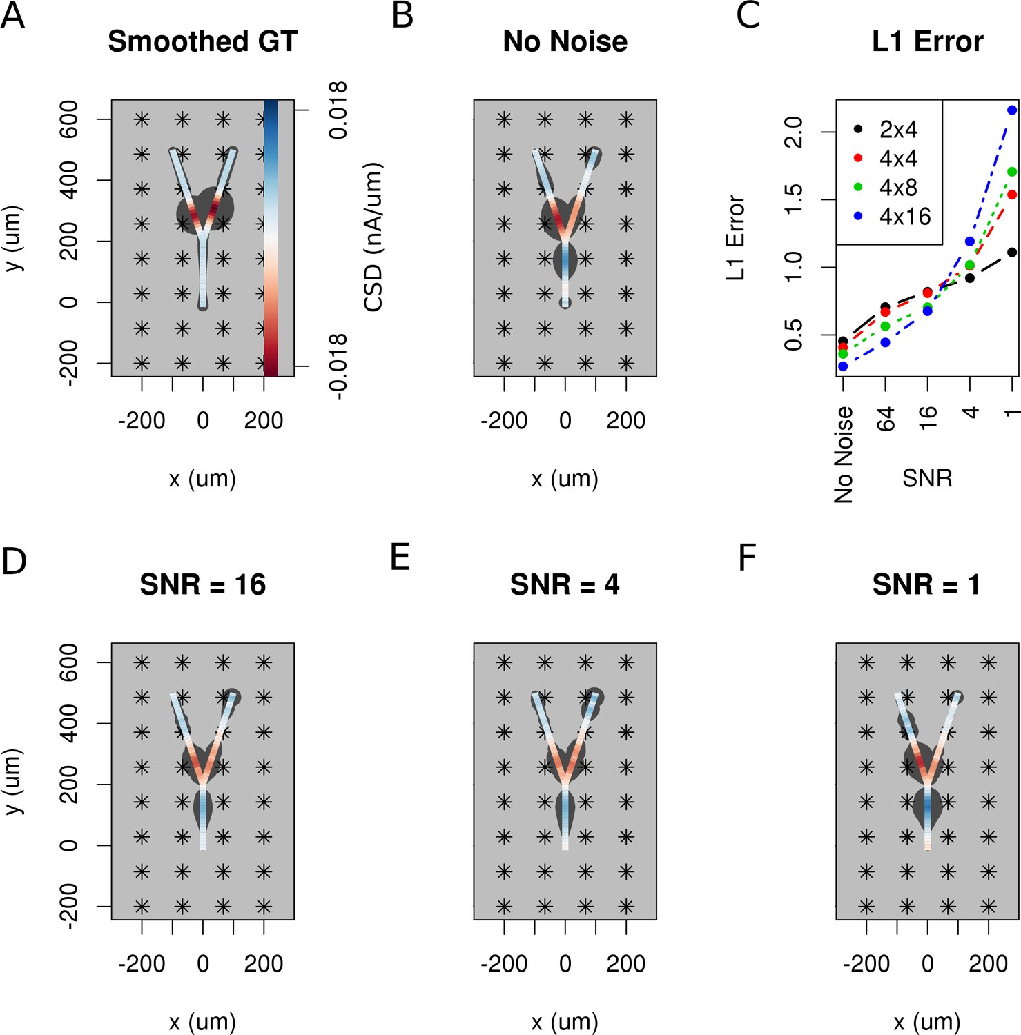
The effect of noise on the reconstruction.
The corrupting influence of noise on the skCSD reconstruction is shown with the example of simultaneous excitation of both branches of the Y-shaped cell close to the branching point in case of the 4 × 8 electrodes setup. (A) Smoothed ground truth CSD shown on the branching morphology used. (B,D,E,F) skCSD reconstructions in cases of no added noise and signal-to-noise ratio equal to 16, 4, 1, respectively. Even the highest noise considered does not fully disrupt the reconstructed source distribution, although increasing the noise systematically degrades the result. This is shown in C, where the L1 error of the reconstruction was calculated for the full length of the simulations. This is consistent for different electrode setups which are marked with various colors. While the setups consisting of more electrodes perform better for low noise, the reconstruction seems to be more sensitive to noise in these cases. This might be a side effect of a specific definition of error.
Figure 10
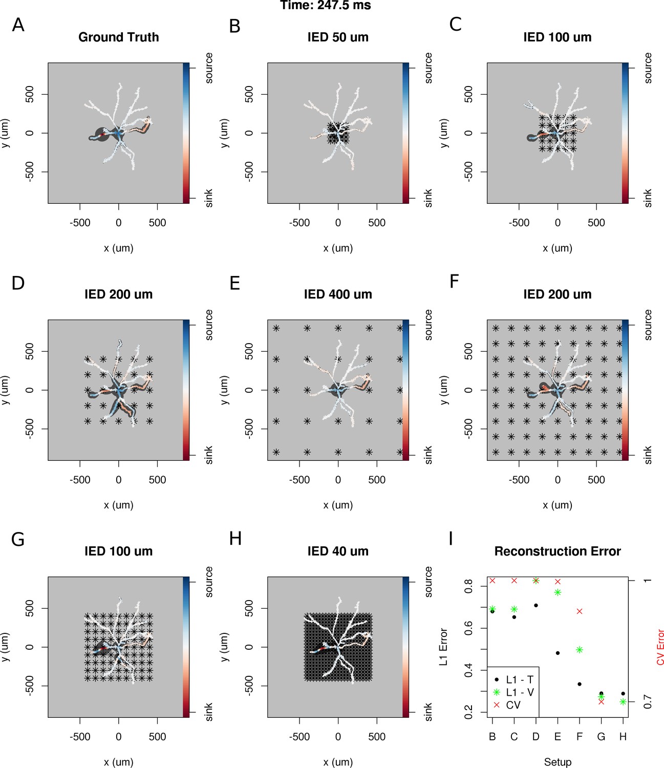
Dependence of skCSD reconstruction on multielectrode setup.
Figures (A–H) show morphology used in the simulation together with the distribution of current sources in branching morphology representation taken at 247.5 ms of the simulation. Figures (B–H) show additionally the electrode setup assumed. (A) Smoothed ground truth CSD. (B) Reconstructed sources for a setup of 5 × 5 electrodes with 50 μm interelectrode distance (IED) covering a small part of the cell morphology around the soma. (C) Reconstructed sources for a setup of 5 × 5 electrodes with 100 μm IED covering a substantial part of the dendritic tree, which improves the reconstruction of the synaptic input on the left. (D) Reconstructed sources for 5 × 5 setup with 200 μm IED setup; both sinks in the membrane currents are visible. (E) Expanding the 5 × 5 electrode setup to 400 μm IED leads to a small number of electrodes placed in the vicinity of the cell which leads to a poor reconstruction. (F) Increasing the number of electrodes to 9 × 9 while keeping the coverage, which leads to 200 μm IED, does not improve the reconstruction. (G) Reducing IED in the previous example to 100 μm, which reduces the coverage of the MEA to the whole cell (same area as in panel D) bringing majority of the electrodes close to one of the dendrites, leads to one of the most faithful reconstructions among the ones shown in this figure. (H) Shows results for a matrix of 21 × 21 contacts with 40 μm IED, covering the same area as in examples D and G. The results are very good but the improvement in reconstruction does not justify the use of so many contacts with so high density. (I) Comparison of reconstruction errors for all the cases shown. Left axis: L1 error for the training (L1–T) and validation (L1–V) part . Right axis: crossvalidation error (CV). The L1-T error is marked with black points, L1-V error is represented by green stars. Generally, the L1-V errors are a bit higher than the L1-T errors but show a similar tendency. Also the CV errors, which are drawn with red crosses, show a similar tendency. The reconstructions in panels (B–H) are for parameters determined with the L1-T error.
Figure 11
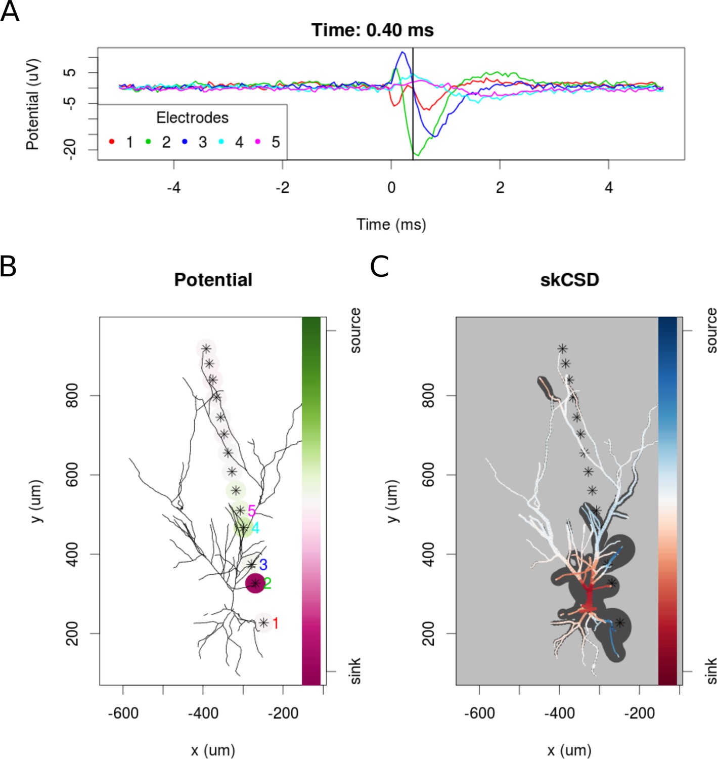
skCSD reconstruction of spike-triggered average for a hippocampal pyramidal cell (A) Extracellular potentials measured with the five electrodes closest to the soma.
The 0 s marks the time of the membrane potential crossing the 0 mV threshold. The black vertical line marks the 0.40 ms time instant for which the extracellular potentials and skCSD reconstruction are shown. (B) Two-dimensional projection of the cell morphology and extracellular electrodes’ positions marked by stars, the five electrodes used in the top panel of the figure are labeled with matching colors. The amplitudes of the measured potentials are shown as color-coded circles around the electrodes. (C) The skCSD reconstruction on the branching morphology representation. This is a snapshot of the cell firing, the red color indicates the sinks close to the soma, the blue marks the current sources on the dendrites.
Author response image 1
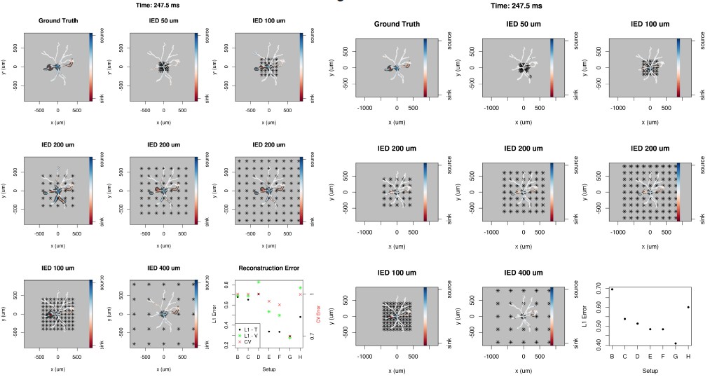
Author response image 2

40 current source density distribution patterns on the Y-shaped morphology: ground truth, skCSD reconstruction from 4x4 and 4x16 electrodes, and the L1 error for each pattern.
The optimal parameters for the skCSD reconstruction were chosen by cross-validation for the whole series of patterns. The reconstruction error is higher for patterns with sharp peaks, in this case the skCSD method smooths these peaks in space.
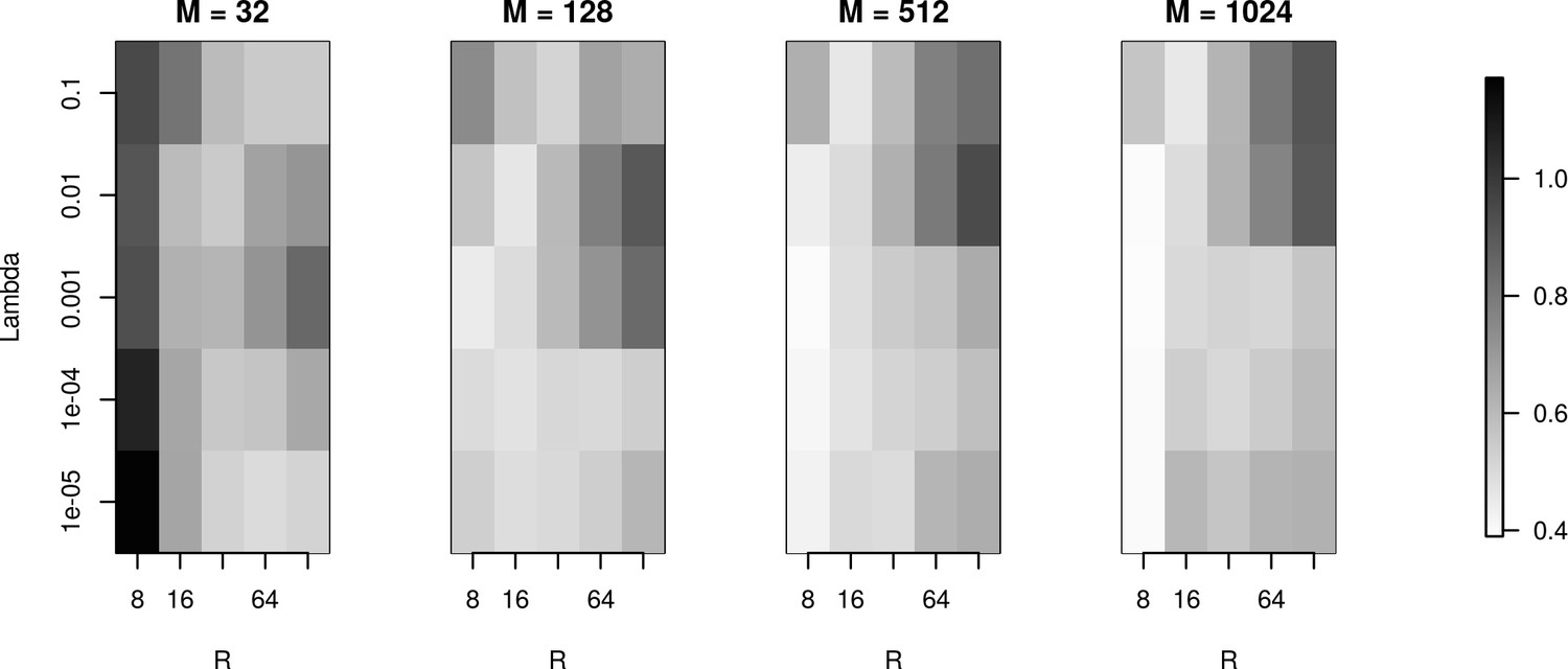
Author response image 3
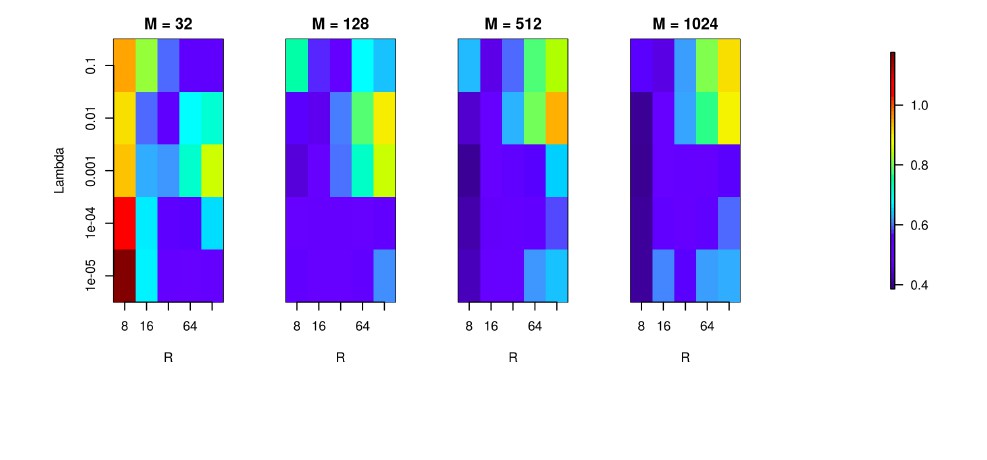
We used the Y-shaped morphology and the 4x4 electrode setup to investigate the effect of using various basis numbers for the reconstruction.
L1 error was calculated to compare the results for basis with 32, 128, 256, 512, 1024 elements (M), for several values of basis width (R) and λ. As shown, using few and narrow basis functions can lead to poor reconstruction, but covering the morphology with a sufficient number of basis functions of reasonable width (on the order of L/M with L being the total dendritic length) significantly improves the reconstruction (reduces the error).
Videos
Video 1
skCSD reconstruction of current source density distribution on the ganglion cell.
The video shows the skCSD reconstruction for the retinal ganglion cell model driven with oscillatory current (Section Reconstruction of current distribution on complex morphology) for the whole duration of simulation. Figure 7 shows a snapshot taken at ms from the simulation onset. During the first 400 ms of simulation, apart from somatic drive, 100 excitatory synaptic inputs were randomly distributed along the dendrites. For reconstruction, 128 virtual electrodes were selected from the 936 arranged in a hexagonal grid of 17.5 μm interelectrode distance to record the extracellular potentials. Panel A presents the somatic membrane potential during the simulation. The red line marks the time instant for which the remaining plots were made. The colormap on Panel B shows the extracellular potential interpolated between the simulated measurements computed at the electrodes, which are marked with asterisks. The regular CSD is shown on Panel C, while the spatially smoothed ground truth membrane current is presented on Panel D. Panel E shows the skCSD reconstruction of current source density along the cell morphology from the selected measurements. The dark gray shapes are guides for the eye and are sums of circles placed along the morphology with radius proportional to the amplitude of the sources at the center of the circle.
Video 2
Spike triggered average of pyramidal cell in vitro.
The video shows the recorded potentials and skCSD reconstruction for a 10 ms time window centered around the spike as described in Section Proof-of-Concept experiment: Spatial Current Source Distribution of Spike-triggered Averages. The top panel presents the spike triggered averages of the potentials during 5 s before and after the spike recorded at five electrodes closest to the soma. The lower left panel shows the morphology of the cell, electrode positions, and the recorded potentials. The electrodes are marked by stars and the amplitude of the recorded potential is shown as color-coded circles around the electrodes. The snapshot is taken at the time given in the figure title and indicated by the black vertical line in the top panel. The reconstructed skCSD distribution at the same moment is shown in the lower right panel. At -0.05 ms a sink appears at the basal dendrites. This can be a consequence of the activation of voltage-sensitive channels in the axon hillock or the first axonal segment leading to the firing of the cell. Since there were no electrodes close to the axon initial segment, the skCSD method did not resolve it, instead it resolved to introduce the activity into the basal dendrite. This phenomenon is quickly replaced by a sink at the soma and in the proximal part of the apical dendritic tree, accompanied by sources (blue) in the basal and in the more distal apical dendrites. The extracellular potential on the second electrode reaches its minimum at 0.45 ms, which signals the peak of the spike. The deep red of the soma at this point signifies a strong sink, while the blue of the surrounding parts of the proximal apical and basal dendrites indicates the current sources set by the return currents. At 1.30 ms a source appears at the soma region, which indicates hyperpolarizing currents.
Tables
Key resources table
| Reagent type (species) or resource | Designation | Source or reference | Identifiers | Additional information |
|---|---|---|---|---|
| Strain, strain background (Wistar rat, male) | Male Wistar rat | PMID: 11619935 | ||
| Biological sample (Wistar rat, male) | Hippocampal slice | |||
| Chemical compound, drug | Biocytin | PMID: 17990268 | ||
| Software, algorithm | Neurolucida Stereo Investigator | PMCID: PMC3332236 | RRID:SCR_001775 | |
| Software, algorithm | RHD2000-Series Amplifier Evaluation System Intan Technologies, LLC | Intan Technologies,http://intantech.com/aboutus.html | ||
| Software, algorithm | LFPy | doi: 10.3389/fninf.2013.00041 | RRID:SCR_014805 | |
| Software, algorithm | NEURON | https://neuron.yale.edu/neuron/ | RRID:SCR_005393 | |
| Software, algorithm | Python Programming Language | http://www.python.org | RRID:SCR_008394 | |
| Software, algorithm | R Project for Statistical Computing | https://www.r-project.org/ | RRID:SCR_001905 | |
| Software, algorithm | NeuroMorpho.Org | PMCID: PMC2655120, http://neuromorpho.org/ | RRID:SCR_002145 | |
| Software, algorithm | Kernel Current Source Density Python library | PMID: 22091662 | RRID:SCR_015777 | |
| Software, algorithm | skCSD method | this paper, https://github.com/csdori/skCSD | A tool for estimating transmembrane currents along the dendritic tree of a neuron from extracellular recordings | |
| Other | Ganglion cell morphology | PMID: 20826176, http://neuromorpho.org/neuron_info.jsp?neuron_name=Badea2011Fig2Du |
Table 1
Main parameters of the simulated cells and setups.
https://doi.org/10.7554/eLife.29384.015| Cell properties | Synapse properties | Distribution of electrodes | |||||
|---|---|---|---|---|---|---|---|
| Length (m ) | Number of Seg. | Location (ID of Seg.) | Number of Syn. | Synaptic Weight (S ) | Type | Number | |
| BS | 516 | 53 | random | 100 | 0.01 | linear | 8,16, 32, 64, 128 |
| Y | 848 | 86 | 33, 62 | 6 | 0.04 | rectangular, random | 2 × 4, 4 × 4, 4x8, 4x16 |
| Y-rot | 848 | 86 | 33, 62 | 6 | 0.04 | rectangular | 8,16, 32, 64 |
| Gang | 5876 | 608 | random | 100 | 0.01 | hexagonal, rectangular | 128, 25, 49, 81, 441 |
Table 2
Biophysical parameters characterizing the simulated cell models.
https://doi.org/10.7554/eLife.29384.016| Quantity | Value | Unit |
|---|---|---|
| Initial potential | −65 | |
| Axial resistance | 123 | |
| Membrane resistivity | 30000 | |
| Membrane capacitance | 1 | |
| Passive mechanism reversal potential | −65 |
Additional files
-
Transparent reporting form
- https://doi.org/10.7554/eLife.29384.017
Download links
A two-part list of links to download the article, or parts of the article, in various formats.
Downloads (link to download the article as PDF)
Open citations (links to open the citations from this article in various online reference manager services)
Cite this article (links to download the citations from this article in formats compatible with various reference manager tools)
Revealing the distribution of transmembrane currents along the dendritic tree of a neuron from extracellular recordings
eLife 6:e29384.
https://doi.org/10.7554/eLife.29384


