Signal integration at spherical bushy cells enhances representation of temporal structure but limits its range
- University of Iowa, United States
- University of Leipzig, Germany
- Radboud University, Netherlands
Figures
Figure 1
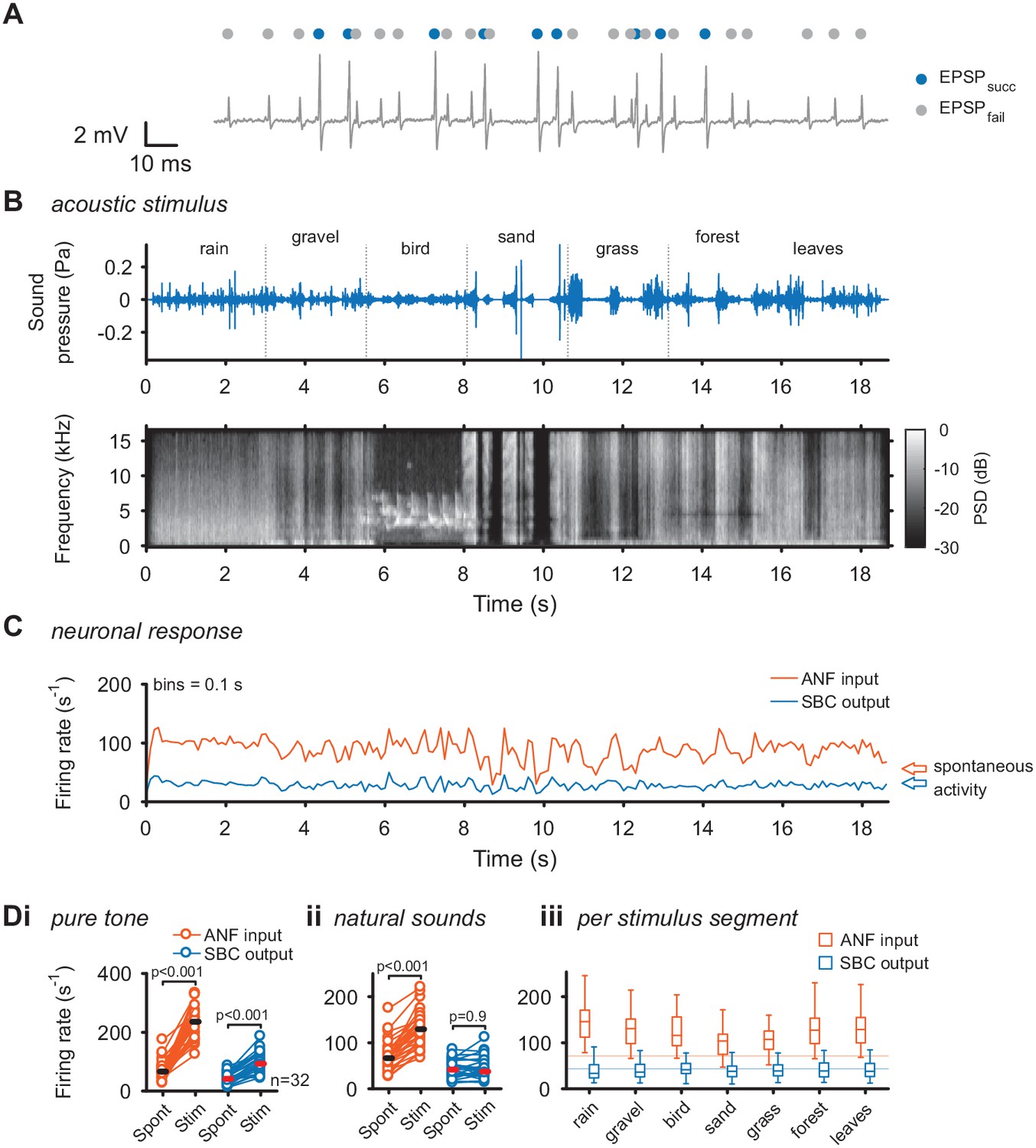
Acoustic stimulation with environmental sounds increases auditory nerve firing while leaving the SBC firing rates constant.
(A) Representative voltage trace of SBC recording during acoustic stimulation. Voltage signals could be divided into EPSP followed by postsynaptic AP (blue dots) and EPSPs which fail to trigger an AP (gray dots). The sum of both types of events comprised the ANF input. (B) The acoustic stimulus was composed of a series of environmental sounds (i.e. rain falling, walking on gravel, bird singing, shoveling sand, ripping grass, walking through forest, walking on fallen leaves), containing naturally occurring frequency and amplitude modulations. Top: amplitude profile; bottom: spectrogram. The stimulus was presented at a mean sound pressure level of 40 dB SPL. PSD = power spectral density. (C) Firing rates of one representative cell during acoustic stimulation (CF = 2.6 kHz, bin size 0.1 s). Note that the firing rate fluctuations at the ANF level (orange) are higher than at the SBC level (blue). Arrows at the right indicate spontaneous firing rates in the absence of sound. (D) Population data on firing rate changes for ANF input and SBC output during pure tone and natural sound stimulation. (i) Pure tone stimulation at the units’ characteristic frequency resulted in a firing rate increase in both ANF input and SBC output. (ii) While during stimulation with natural sounds, the average ANF firing increased comparably to pure tone stimulation, the average SBC firing remains at the level of spontaneous activity. (iii) This effect was consistently observed throughout different stimulus segments of the natural sound stimulus. Horizontal lines indicate the average spontaneous firing rate in the absence of sound.
-
Figure 1—source data 1
Firing rates of auditory nerve (ANF) input and Spherical Bushy Cell (SBC) output during spontaneous activity, pure tone and natural acoustic stimulation.
Data are in Hz.
- https://doi.org/10.7554/eLife.29639.003
Figure 2 with 1 supplement
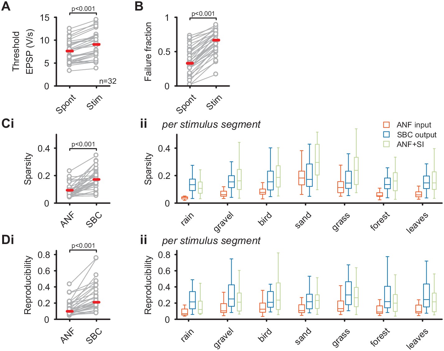
SBC output exhibits increased sparsity and reproducibility compared to ANF input which can be attributed to activity-dependent subtractive inhibition.
(A) During acoustic stimulation the threshold EPSP for AP generation (left) was increased and consequently so was the failure fraction (right), indicating strong inhibition during acoustic stimulation with natural sounds. (B) (i) The sparsity of the neuronal response was separately calculated for the ANF input and the SBC output. The SBC output showed consistently higher sparsity than the ANF input. (ii) The increase in sparsity from the ANF input (orange) to the SBC output (blue) was consistently observed for the different stimulus segments. Simulated (subtractive) inhibition (ANF +SI, green) resulted in similar increases in sparsity. Notably, for conditions in which the sparsity of the ANF input was high (i.e. 'sand'), the SBC output did not increase further. (C) (i) Similar to sparsity, the reproducibility of the neuronal response increased at the SBC level. (ii) Again, this effect was consistent for the different stimulus segments and well approximated by simulating subtractive inhibition.
-
Figure 2—source data 1
Threshold EPSP (in V/s) and failure fraction during acoustic spontaneous activity and natural acoustic stimulation.
Values of sparsity and reproducibility for ANF input and SBC output for both the complete stimulus and separated in stimulus segments.
- https://doi.org/10.7554/eLife.29639.007
Figure 2—figure supplement 1
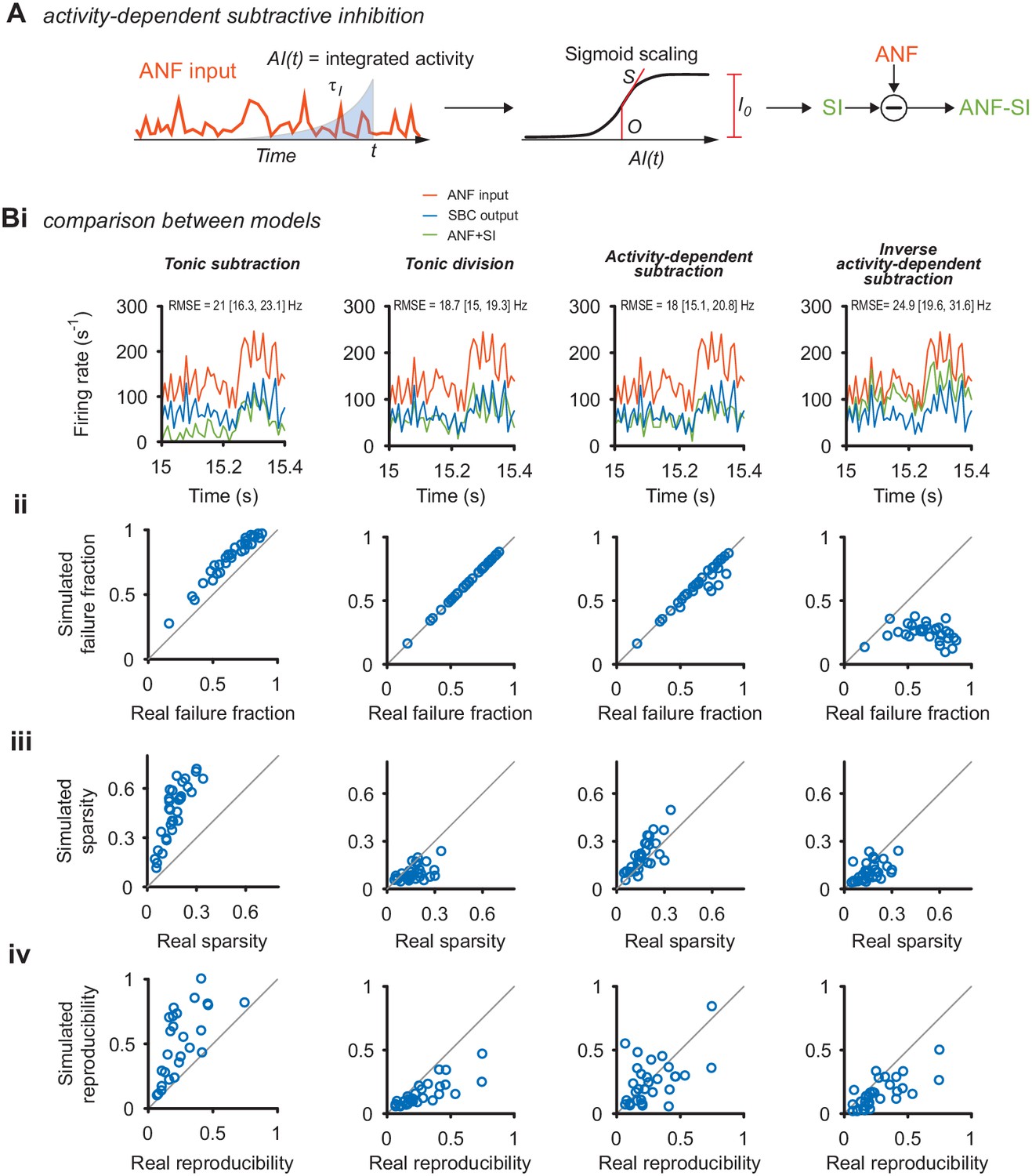
Comparison of different inhibition models in their ability to reproduce the response as well as its sparsity and reproducibility.
(A) Schematic of the activity-dependent subtractive inhibition (ADSI) model. The PSTH of the ANF input was time-shifted and integrated with an exponential kernel with time-constant to obtain an intermediate representation AI(t). The resulting signal was passed through a static, sigmoid nonlinearity defined by the slope S, the instantaneous strength of inhibition I0, and the midpoint O. The resulting function is then subtracted from the experimental ANF input to obtain the PSTH with simulated inhibition (ANF +SI). The strength of inhibition was adjusted for each cell to match the experimentally observed failure rates. (B) Several models of inhibition could account for the observed responses, quantified as the failure fraction (ii), sparsity (iii), reproducibility (iv) and the RMSE. The quality of the ADSI model was then compared to three other models of inhibition: tonic subtractive inhibition (left column), tonic divisive inhibition (middle left), and an inverse activity-dependent inhibition (right). (i) PSTH sections of a representative cell (CF = 1.8 kHz) for the ANF input (orange), SBC output (blue) and the simulated SBC output after applying the respective inhibition model (ANF +SI, green). Both divisive (middle left) and ASDI (middle right) showed good overlap with the experimental SBC output and with a margin displayed the lowest absolute squared error (RMSE) between data and model. (ii) Divisive inhibition and ASDI matched the experimental failure rates well. Pure subtraction (left) resulted in slight overestimation and inverse activity-dependent inhibition failed to reach the experimentally observed failure rates. (iii) The increase in sparsity was best matched with the ASDI model. Tonic subtraction resulted in sparsity exceeding the experimental data, while divisive inhibition and inverted ASDI failed to increase sparsity. (iv) The increase in reproducibility was overestimated in the tonic subtraction model and underestimated in the divisive inhibition and inverse ASDI. The ASDI model showed on average a qualitatively good fit with the data, with some cells being under- or overestimated. Overall the ADSI model showed the best combination of match with the real data along the compared dimensions.
Figure 3 with 1 supplement
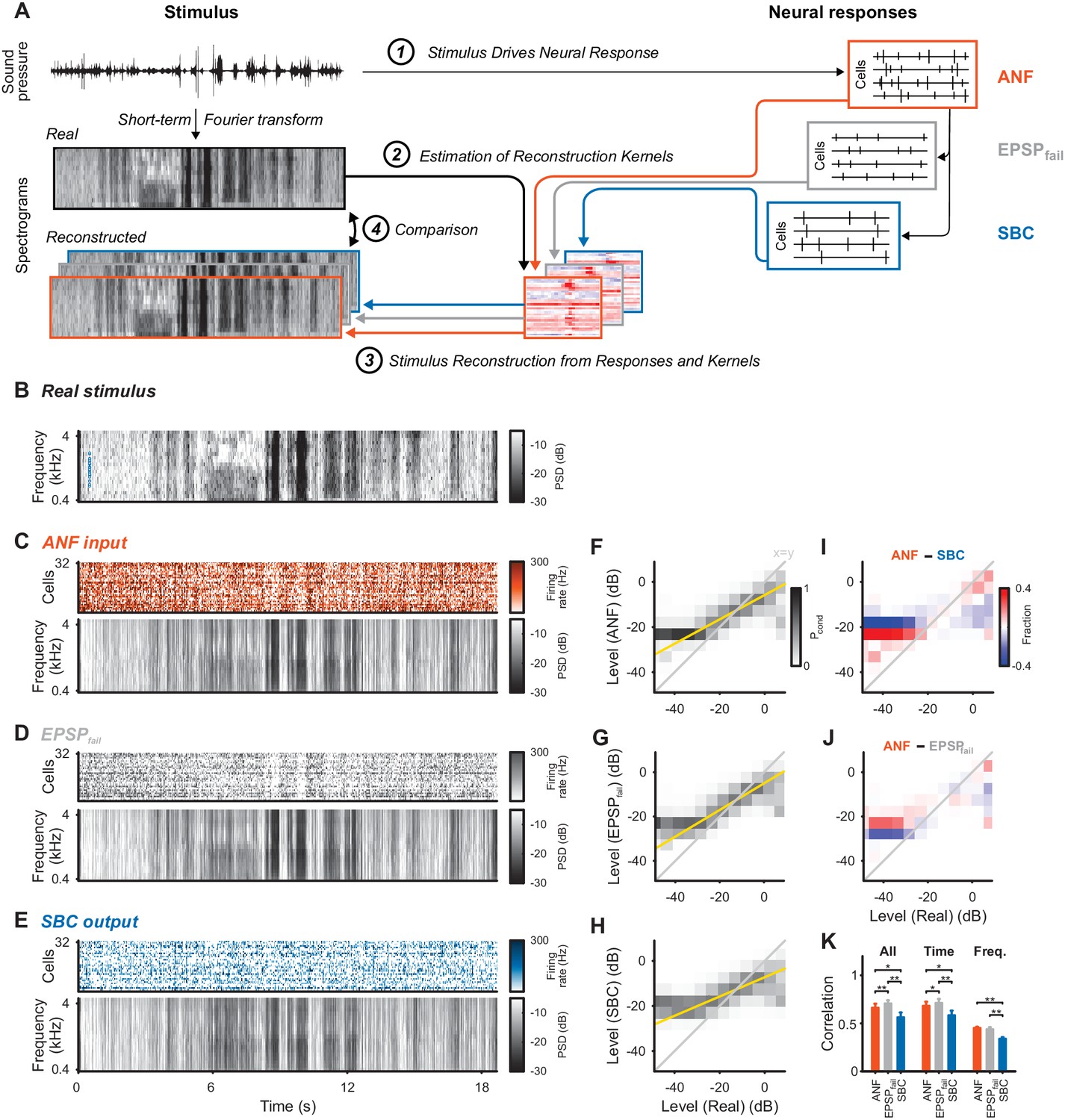
Stimulus representation in the SBC responses is less accurate than in the ANF activity or in the inhibited EPSPs (EPSPfail).
(A) Stimulus reconstruction was performed by estimating linear reconstruction kernels (2) for ANF-, EPSPfail- and SBC responses (1), separately. The respective reconstructions were then used to predict stimulus reconstructions (3), which were then compared to the real stimulus used in the estimation (4). (B) Spectrogram of the real stimulus. The frequency range was reduced from its original range of 16 kHz (see Figure 1B) to the range represented in the ANFs’ receptive fields (0.3–4.4 kHz, CFs shown as blue dots on the left). Color scales are identical for all spectrograms. PSD = power spectral density. (C) The population response of the ANFs sorted by CF (top) and the ANF-reconstructed stimulus (bottom). The global structure and even the envelope fine-structure is preserved in the reconstruction. For more finely resolved spectrograms see Figure 4. (D) The rate of EPSPfail sorted as above (top) and the EPSPfail-reconstructed stimulus (bottom). Again, global structure and envelope fine-structure are preserved with inaccuracies in the overall range. (E) The SBC AP population response (top) and the SBC-reconstructed stimulus (bottom). While the envelope fine-structure appears again preserved, the range of the reconstruction is much more limited, i.e. relatively faint parts appear louder in the reconstruction louder than expected (e.g. around 9 s), and vice versa loud parts appear fainter (e.g. after 6 s). (F) The joint histogram across levels between real (abscissa) and reconstructed (ordinate) for ANF responses. The correlation between the two is evident (compare to grey diagonal representing x = y), with a slight deviation below −23 dB, were the reconstructed stimulus did not cover low enough levels (yellow line indicates linear regression). (G) The EPSPfail-based joint histogram with true level exhibits an overall similar shape as the SBCs (see panel J for detailed comparison). (H) The SBC-based joint histogram is more widely distributed around the diagonal and limited in range (see panel I for detailed comparison). (I) Subtraction of the SBC-based from the ANF-based histogram indicates an increase in width apparent by the negative (blue) margins and the positive (red) spine. (J) Subtracting instead the EPSPfail-based from the ANF-based histogram, leads to a much smaller difference with an even better correlation around the diagonal for EPSPfail (blue parts on diagonal) for low and high levels. (K) The correlation between the real and the reconstructed stimulus was significantly worse for SBCs compared with either ANF or EPSPfail. Correlation was mostly governed by temporal (middle), rather than spectral (right) variations for all three signals (n = 10 cross-validation sections, based on 32 neurons, *p<0.05, **p<0.01, see Table 1 for exact p-values).
-
Figure 3—source data 1
Correlation between real acoustic and reconstructed stimulus based on ANF input, SBC output and EPSPfail signals.
- https://doi.org/10.7554/eLife.29639.010
Figure 3—figure supplement 1
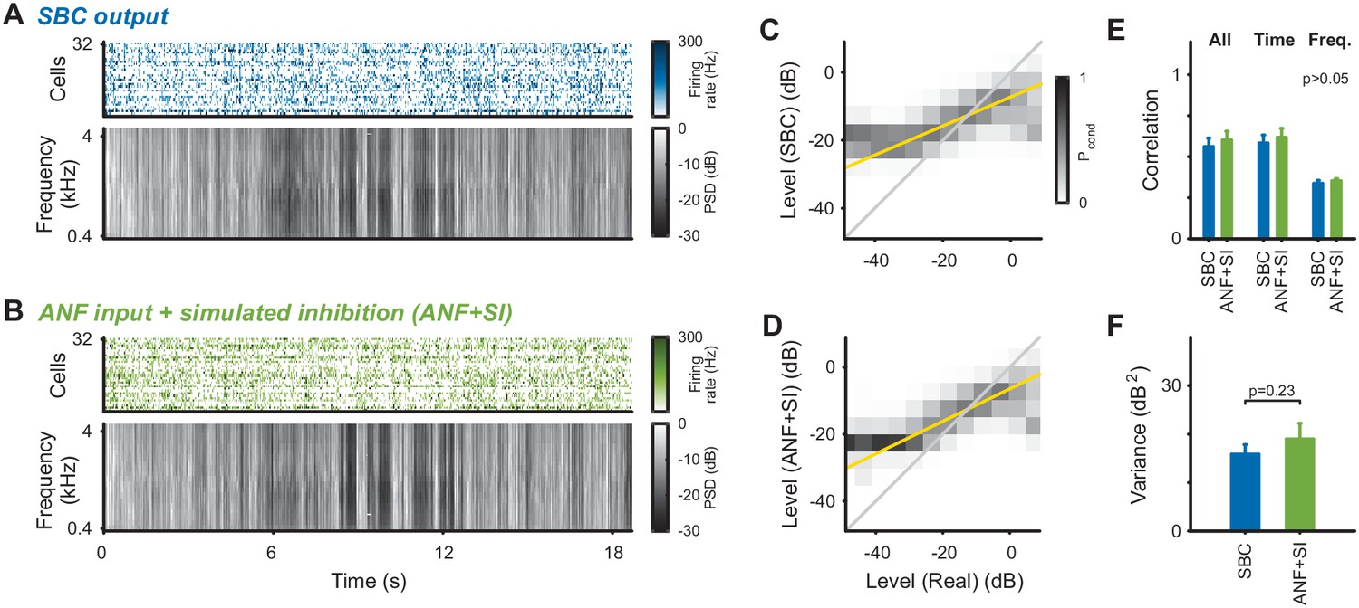
For certain postsynaptic response properties, the effect of inhibition appears to be accounted for well by activity-dependent subtractive inhibition (Figure 2, and Keine et al., 2016).
We compared the stimulus reconstruction between the experimental SBC output and the ANF input subject to same subtractive inhibition as in Figure 2 (ANF + SI, see Materials and methods for details). (A) SBC responses and reconstructed spectrogram, same as Figure 3E, provided for direct comparison. (B) Subtractive inhibition applied to the ANF responses (ANF + SI) leads to similar responses and reconstructed spectrogram as for the SBC responses. (C) Joint histogram of reconstructed levels from SBC responses compared with the real levels (as in Figure 3H). (D) Joint level histogram comparing the ANF + SI to the real levels, take a similar shape with almost identical slope compared to the SBC responses. However, SBC responses have an even more restricted dynamic range for low levels. (E) Reconstruction quality measured by correlation coefficients did not differ significantly between SBC and ANF + SI for either total, time or frequency correlations (all p>0.05). (F) Variance of the reconstructed stimulus for ANF + SI was comparable to the experimental SBC output (p=0.23).
Figure 4

Envelope fine-structure properties of the reconstructed stimulus differ between ANF and SBC responses.
(A) A 250 ms snippet of the real spectrogram (Figure 3B) zoomed in. The yellow box indicates a region for comparing the across frequency correlations across the different spectrograms (see G). (B) The reconstructed stimulus from the ANFs shows that temporal features of the stimulus can be reconstructed down to approximately 5–10 ms (visual estimate), which is coarser than the resolution of the spectrogram (2 ms). (C) The EPSPfail reconstruction appears similar to the ANF reconstruction, with an overall smoother appearance. (D) The SBC reconstruction appears more ‘vertical’, that is, with more correlation across frequencies (see G) and less modulation, but otherwise temporally sharp (see E). (E) The temporal precision of the different reconstructions was assessed by the width of the autocorrelation (inset: width of peak), resolved at multiple heights (inset: horizontal lines, black to red) relative to the correlation at Δt = 0 (inset: maximum). The SBC (blue) reconstruction was most precise, while the EPSPfail (grey) was least precise (2-way ANOVA with factors ‘relative height’ and ‘response type’, see panel for p-values, n = 10 stimulus sections). (F) The emphasis of the temporal modulations was overall similar with a significant overrepresentation of the 100–160 Hz in the SBC reconstruction (PSD = power spectral density, 2 SEM shown, however, very small variation, see panel for p-values, black dots indicate regions of significant deviation with False-Discovery-Rates at p<0.001, Benjamini and Hochberg, 1995). (G) The spectral correlation of SBC was larger than for ANFs and EPSPfail for large frequency separations (>2 kHz, see panel for p-values). Correlations were computed for different frequency separations (abscissa), but within each time-bin.
-
Figure 4—source data 1
Properties of the reconstructed stimulus based on ANF, SBC and EPSPfail activity.
- https://doi.org/10.7554/eLife.29639.012
Author response image 1
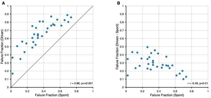
Relation between spontaneous and driven failures.
(A) Acoustically driven failure rates always exceeded spontaneous failures, but correlated well with each other. This suggests that the effects of spontaneous failures and stimulus-driven failures (by inhibition or otherwise) are 'additive', although we cannot discern, whether this is true addition (i.e. FF(s + d) = FF(s) + FF(d)) or just a 'greater than' relation (i.e. FF(s+d) > FF(s)). (B) The additional failures during stimulation (i.e. Driven – Spontaneous) showed a slight negative correlation. We think this dependence is expected, since in units with higher spontaneous failure fractions, only a smaller fraction of successful transmission events remains, that can still fail during stimulation.
Tables
Table 1
Summary of statistical comparisons.
https://doi.org/10.7554/eLife.29639.004| Source | Parameter | Group 1 (mean ± SD) | Group 2 (mean ± SD) | Test statistics | Statistical test |
|---|---|---|---|---|---|
| Figure 1 | |||||
| Panel Di (pure tones) | Firing Rate ANF | Spont = 71.3 ± 31.8 Hz | Stim = 234.3 ± 53.9 Hz | t(df = 31) = –15.5, p=3.5e-16, U1=0.87 | paired t test |
| Firing Rate SBC | Spont = 43.4 ± 18.3 | Stim = 97.3 ± 33.9 | t(31) = –10.9, p=3.5e-12, U1=0.59 | paired t test | |
| Panel Dii (natural sounds) | Firing Rate ANF | Spont = 71.3 ± 31.8 Hz | Stim = 129.7 ± 38.4 Hz | t(31) = –12.9, p=4.9e-14, U1=0.3 | paired t test |
| Firing Rate SBC | Spont = 43.4 ± 18.3 | Stim = 43.1 ± 22.1 | t(31) = 0.12, p=0.9, U1=0.03 | paired t test | |
| Figure 2 | |||||
| Panel A | Threshold EPSP | Spont = 7.5 ± 2.4 V/s | Stim = 9 ± 2.8 V/s | t(31) = –10.2, p=1.8e-11, U1=0.1 | paired t test |
| Panel B | Failure Fraction | Spont = 0.36 ± 0.2 | Stim = 0.65 ± 0.17 | t(31) = –16.3, p=9.1e-17, U1=0.28 | paired t test |
| Panel Ci | Sparsity | ANF input = 0.09 ± 0.05 | SBC output = 0.17 ± 0.07 | t(31) = –6.9, p=8.2e-8, U1=0.17 | paired t test |
| Panel Di | Reproducibility | ANF input = 0.13 ± 0.09 | SBC output = 0.28 ± 0.18 | Z(N=32) = –4.9, p=8.8e-7, U1=0.2 | Wilcox. sig.-rank |
| Figure 3 | |||||
| Panel K | Corr. Section | ANF = 0.66 ± 0.14 | EPSP = 0.71 ± 0.11 | Z(N=10) = –2.8, p=0.006*, U1=0.1 | Wilcox. sig.-rank |
| Corr. Section | ANF = 0.66 ± 0.14 | SBC = 0.56 ± 0.16 | Z(N=10) = –2.8, p=0.006*, U1=0.1 | Wilcox. sig.-rank | |
| Corr. Section | EPSP = 0.71 ± 0.11 | SBC = 0.56 ± 0.16 | Z(N=10) = 2.8, p=0.006*, U1=0.35 | Wilcox. sig.-rank | |
| Corr. Time Section | ANF = 0.68 ± 0.14 | EPSP = 0.71 ± 0.14 | Z(N=10) = –2.7, p=0.0117*, U1=0.1 | Wilcox. sig.-rank | |
| Corr. Time Section | ANF = 0.68 ± 0.14 | SBC = 0.58 ± 0.15 | Z(N=10) = 2.7, p=0.0117*, U1=0.15 | Wilcox. sig.-rank | |
| Corr. Time Section | EPSP = 0.71 ± 0.14 | SBC = 0.58 ± 0.15 | Z(N=10) = 2.8, p=0.006*, U1=0.25 | Wilcox. sig.-rank | |
| Corr. Freq. Section | ANF = 0.45 ± 0.042 | EPSP = 0.44 ± 0.071 | Z(N=10) = 1.6, p=0.39*, U1=0.2 | Wilcox. sig.-rank | |
| Corr. Freq. Section | ANF = 0.45 ± 0.042 | SBC = 0.34 ± 0.058 | Z(N=10) = 2.8, p=0.006*, U1=0.85 | Wilcox. sig.-rank | |
| Corr. Freq. Section | EPSP = 0.44 ± 0.071 | SBC = 0.34 ± 0.058 | Z(N=10) = 2.8, p=0.006*, U1=0.5 | Wilcox. sig.-rank | |
| Factor 1 | Factor 2 | ||||
| Figure 4 | |||||
| Panel E | Autocorrelation | Height: p=2.9e-25 | Response Type: p=0.002 | ANOVA, 2-factor | |
| Panel F | Spectra | Mod. Rate: p=1.7e-6 | Response Type: p=2.1e-51 | ANOVA, 2-factor | |
| Panel G | Freq. XCorr | Delta Freq: p=1.1e-14 | Response Type p=0.023 | ANOVA, 2-factor | |
-
*p-values Bonferroni-corrected for N = 3 comparisons.
Additional files
-
Source code 1
Calculation of threshold EPSP.
- https://doi.org/10.7554/eLife.29639.013
-
Source code 2
Calculation of reproducibility.
- https://doi.org/10.7554/eLife.29639.014
-
Source code 3
Calculation of sparsity.
- https://doi.org/10.7554/eLife.29639.015
-
Source code 4
Simulation of activity-dependent subtractive inhibition.
- https://doi.org/10.7554/eLife.29639.016
-
Supplementary file 1
Related to Figure 1.
Waveform audio file of presented natural stimulus. The stimulus was presented monaurally at a sampling rate of 97.65625 kHz.
- https://doi.org/10.7554/eLife.29639.017
-
Transparent reporting form
- https://doi.org/10.7554/eLife.29639.018
Download links
A two-part list of links to download the article, or parts of the article, in various formats.
Downloads (link to download the article as PDF)
Open citations (links to open the citations from this article in various online reference manager services)
Cite this article (links to download the citations from this article in formats compatible with various reference manager tools)
Signal integration at spherical bushy cells enhances representation of temporal structure but limits its range
eLife 6:e29639.
https://doi.org/10.7554/eLife.29639


