Paradoxical response reversal of top-down modulation in cortical circuits with three interneuron types
- New York University, United States
Figures
Figure 1
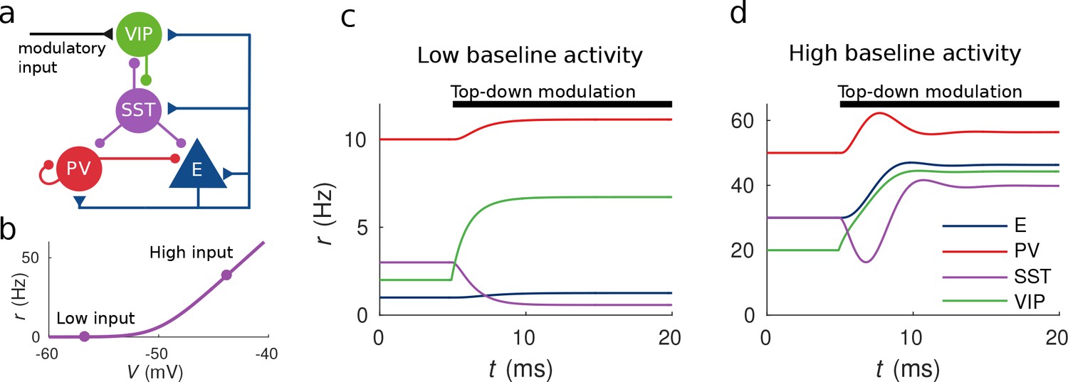
Response to top-down modulation depends on baseline activity.
(a) Microcircuit connectivity and top-down modulatory input. (b) f-I curve. When input is low changes in input have almost no effect on the output rate, instead, when input is high changes in input have a big effect on output rate. (c, d) Transient dynamics upon the onset of the top-down modulatory current for low baseline activity (i.e. when the rates are low before top-down modulation) and high baseline activity (i.e. when the rates are high before top-down modulation). Under a low baseline activity condition, SST is inhibited and E and PV are slightly disinhibited. The high baseline activity condition shows an example of response reversal in SST activity: it initially goes below the baseline rate but due to significant change in E activity and to the recurrent excitation it eventually reverses to a rate higher than baseline.
Figure 2
Response matrix and disinhibition vs. response reversal regime.
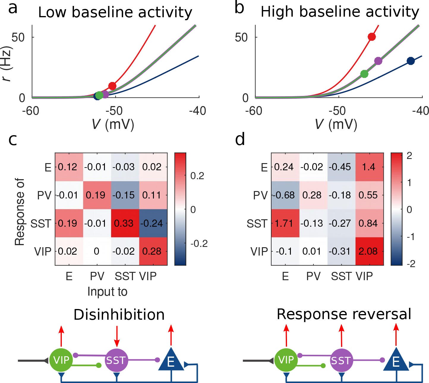
(a–b) Tuning curves for the different populations and baseline activity in both scenarios (low and high). In the low baseline activity scenario (a) all populations are below threshold (flat part of the fI curve), instead in the high baseline activity scenario (b) all populations are above threshold, where small changes in input result in large changes in rate. (c–d) Response matrices for the two scenarios. In (c) the response of SST to external excitation of VIP is negative, while the responses of E and PV are positive. This corresponds to the disinhibition regime. In (d) the responses of all populations to external excitation of VIP are positive, in particular, the response of SST is reversed with respect to (c) corresponding to the response reversal regime.
Figure 3
Random network model.
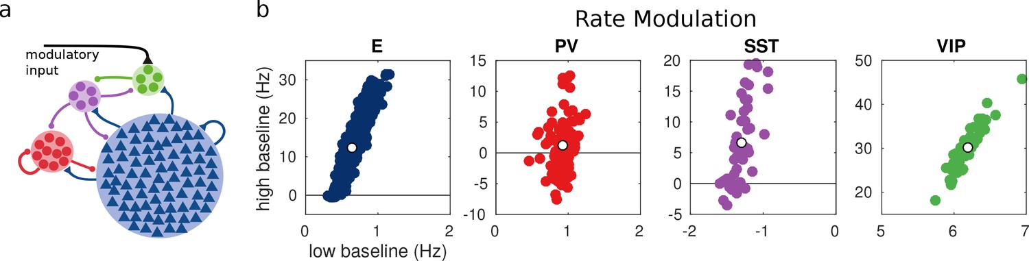
(a) Schematic of the model. Each population is composed of several rate units and the connectivity between units is random with probabilities extracted from experimental data in the literature. (b) Rate modulation (rate after the onset of the modulatory current minus baseline rate) for low and high baseline activities. Each colored point corresponds to one unit. Unit responses are very variable and, in particular within the same population different units might have responses with different sign. White points correspond to the population average. Despite the variability of individual responses the population average corresponds to the population responses in the single unit model in Figure 1.
Figure 4 with 3 supplements
Model of mouse V1 behavior.
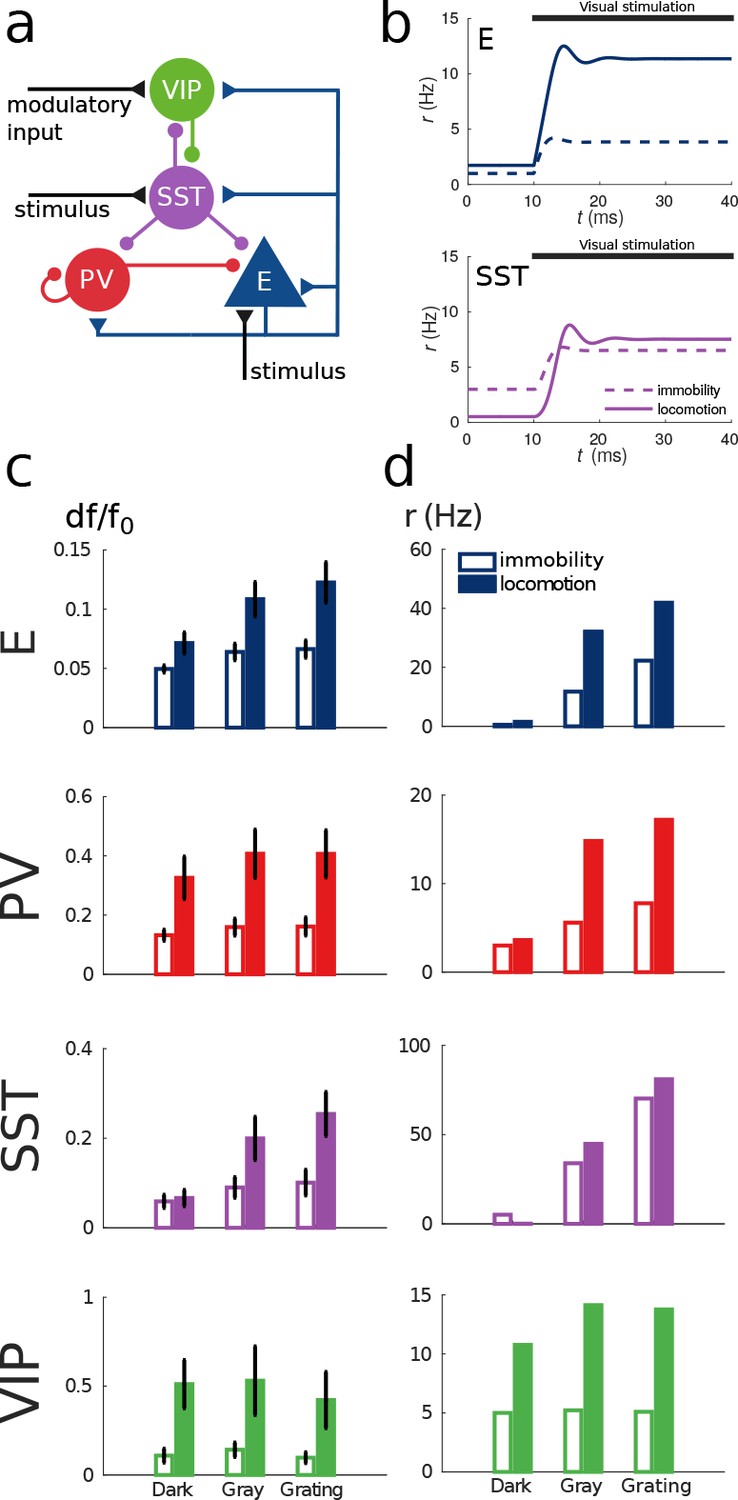
(a) Schematic of the microcircuit. Visual input targets E and SST cells. Behavior related top-down modulation targets VIP cells. (b) Response of E and SST populations when a weak visual stimulus (6 deg) is presented for locomotion and immobility. The E population always shows a higher response with locomotion. On the other hand, before the visual stimulation the SST population has higher activity for immobility than for locomotion and when the visual stimulus is presented, the activity of the SST population is higher for locomotion. (c) Relative change in calcium fluorescence for three levels of visual stimulation (darkness, gray screen and grating) and two behavioral states: immobility (empty bars) and locomotion (filled bars) extracted from Pakan et al. (2016). (d) Rates (in Hz) of the populations in the V1 simulation for the same conditions as in (c). Comparison of (c) with (d) shows that our simulations reproduce qualitatively the activity of neural populations in mice V1. Namely the activity of all populations is higher during locomotion than during immobility whenever there is visual stimulation and for E, PV and VIP also in the absence of visual stimulation. Our model shows a decrease in activity of SST during locomotion as reported in Fu et al. (2014) (the change in activity of the SST population in darkness in Pakan et al. (2016) is not statistically significant). The quantitative differences might be related to the fact that changes in calcium fluorescence are not proportional to changes in rate.
Figure 4—figure supplement 1
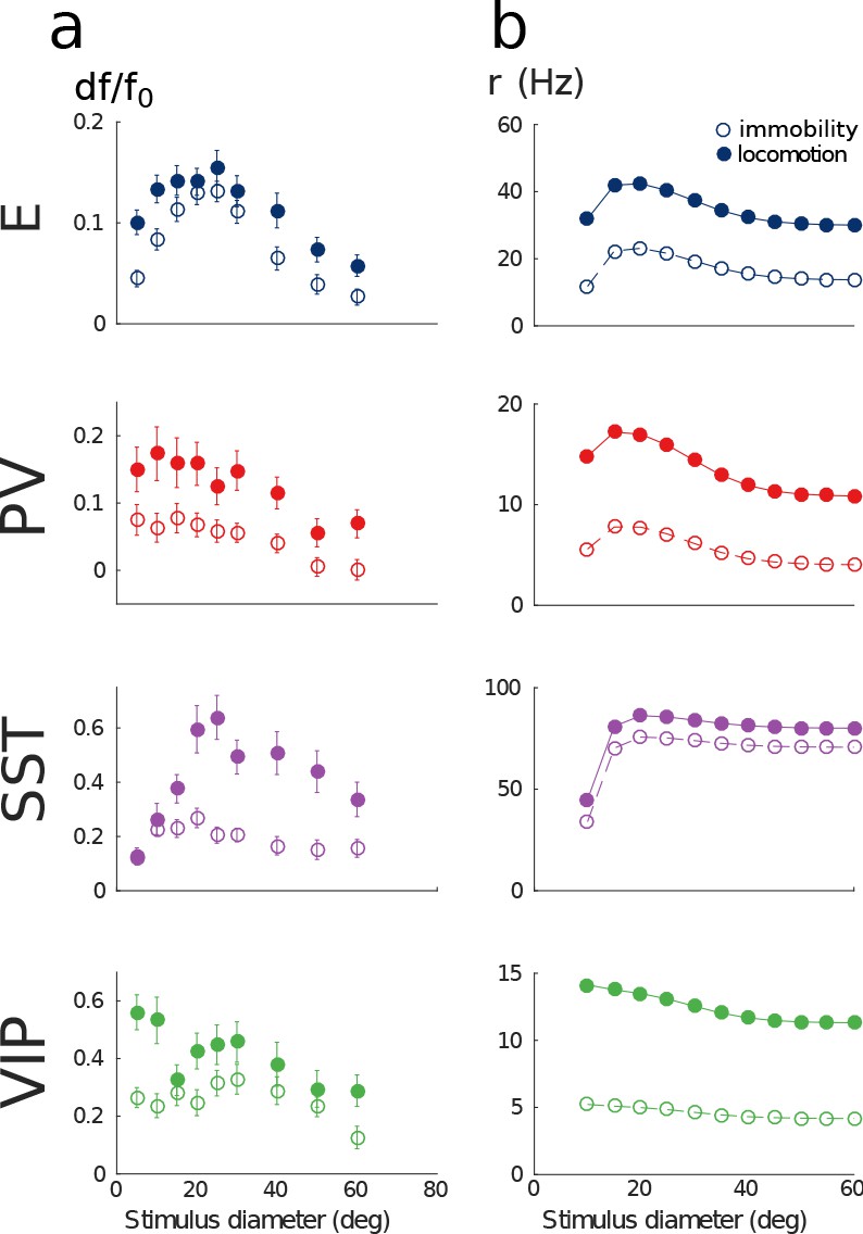
Model of mouse V1 behavior with different grating sizes.
(a) Relative change in calcium fluorescence for gratings of diameters ranging from 10 deg to 60 deg for the two behavioral states: immobility (empty dots) and locomotion (filled dots) extracted from the preprint (Dipoppa et al., 2017) (b) Rates (in Hz) of the populations in the V1 simulation for the same conditions as in (a). As in Figure 4, our simulations reproduce qualitatively the activity of neural populations in mice V1. Our model also exhibits surround suppression for all populations.
Figure 4—figure supplement 2
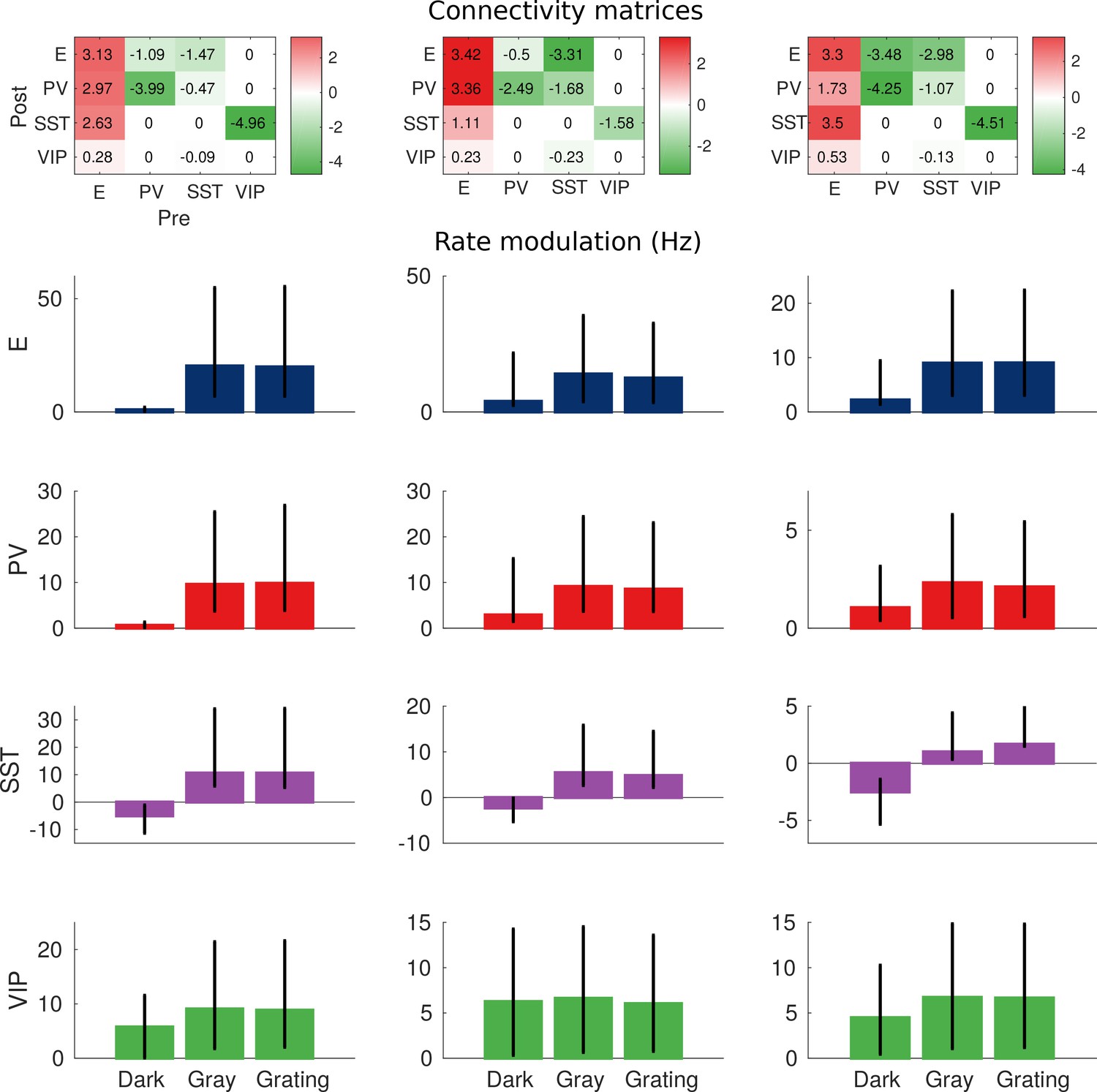
Robustness of the behavior.
Top: Example of three connectivity matrices that have the same qualitative behavior (in pAs). Bottom: rate modulation (rate during locomotion minus rate for immobility). Each bar corresponds to the average rate modulation of 20 random perturbations of the matrices on the top where each entry has been multiplied by a random variable uniformly distributed in , which corresponds to random changes of up to ±10%. Error bars correspond to the minimum and maximum rate modulations of the 20 realizations. Despite quantitative variations, the qualitative behavior is always the same: rate modulation of SST population in darkness is always negative; rate modulation for all other cases is always positive.
Figure 4—figure supplement 3
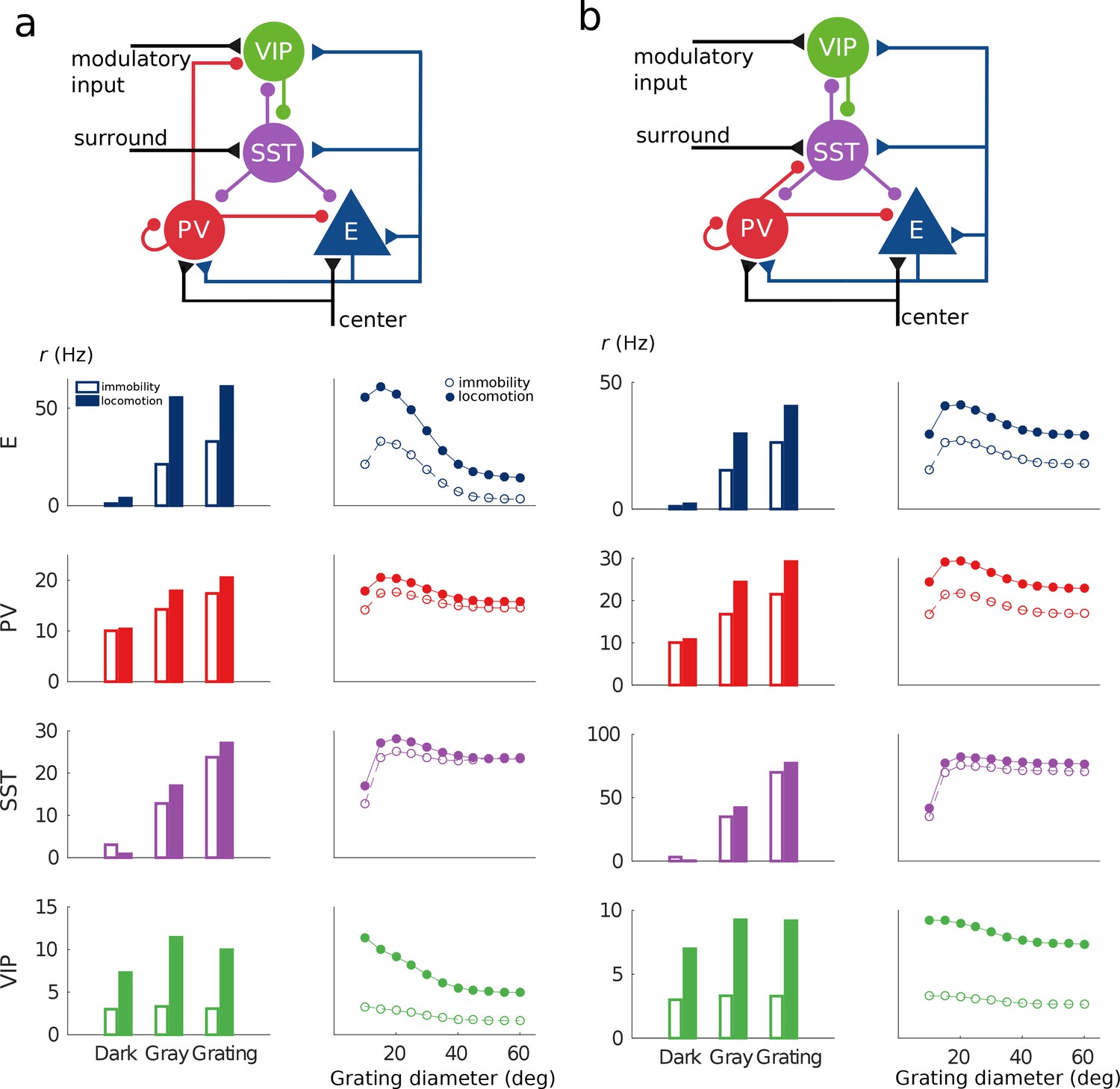
Alternative architectures.
Two alternative microcircuits with visual input targeting E, SST and PV populations and PV to VIP (a) and PV to SST (b) connections exhibit the same qualitative behavior as the circuit in Figure 1 and Figure 4—figure supplement 1.
Tables
Table 1
Connectivity matrix (in pAs).
| From | |||||
|---|---|---|---|---|---|
| E | PV | SST | VIP | ||
| to | E | 2.42 | −0.33 | −0.80 | 0 |
| PV | 2.97 | −3.45 | −2.13 | 0 | |
| SST | 4.64 | 0 | 0 | −2.79 | |
| VIP | 0.71 | 0 | −0.16 | 0 | |
Table 2
Population-dependent parameters.
| E | PV | SST | VIP | |
|---|---|---|---|---|
| 6.25 nS | 10 nS | five nS | five nS | |
| 28 ms | 8 ms | 16 ms | 16 ms |
Table 3
Entries of the respone matrix.
Table 4
Connection probabilities for the random network model.
| From | |||||
|---|---|---|---|---|---|
| E | PV | SST | VIP | ||
| to | E | 0.02 | 1 | 1 | 0 |
| PV | 0.01 | 1 | 0.85 | 0 | |
| SST | 0.01 | 0 | 0 | −0.55 | |
| VIP | 0.01 | 0 | 0.5 | 0 | |
Table 5
Connectivity matrix for the mouse V1 model (in pAs).
| From | |||||
|---|---|---|---|---|---|
| E | PV | SST | VIP | ||
| to | E | 3.30 | −3.48 | −2.98 | 0 |
| PV | 1.73 | −4.25 | −1.07 | 0 | |
| SST | 3.50 | 0 | 0 | −4.51 | |
| VIP | 0.53 | 0 | −0.13 | 0 | |
Additional files
Download links
A two-part list of links to download the article, or parts of the article, in various formats.
Downloads (link to download the article as PDF)
Open citations (links to open the citations from this article in various online reference manager services)
Cite this article (links to download the citations from this article in formats compatible with various reference manager tools)
Paradoxical response reversal of top-down modulation in cortical circuits with three interneuron types
eLife 6:e29742.
https://doi.org/10.7554/eLife.29742


