Figures and data in A high-resolution mRNA expression time course of embryonic development in zebrafish

Figures
Tables
Additional files

12 figures, 3 tables and 20 additional files

Figures

Figure 1 with 2 supplements

Download asset Open asset

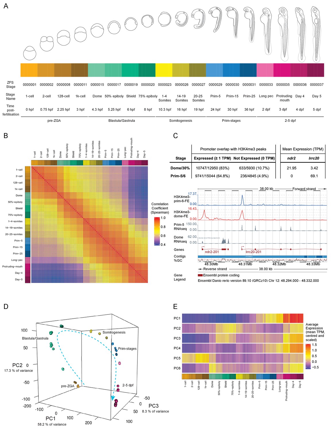
A transcriptional map of development.

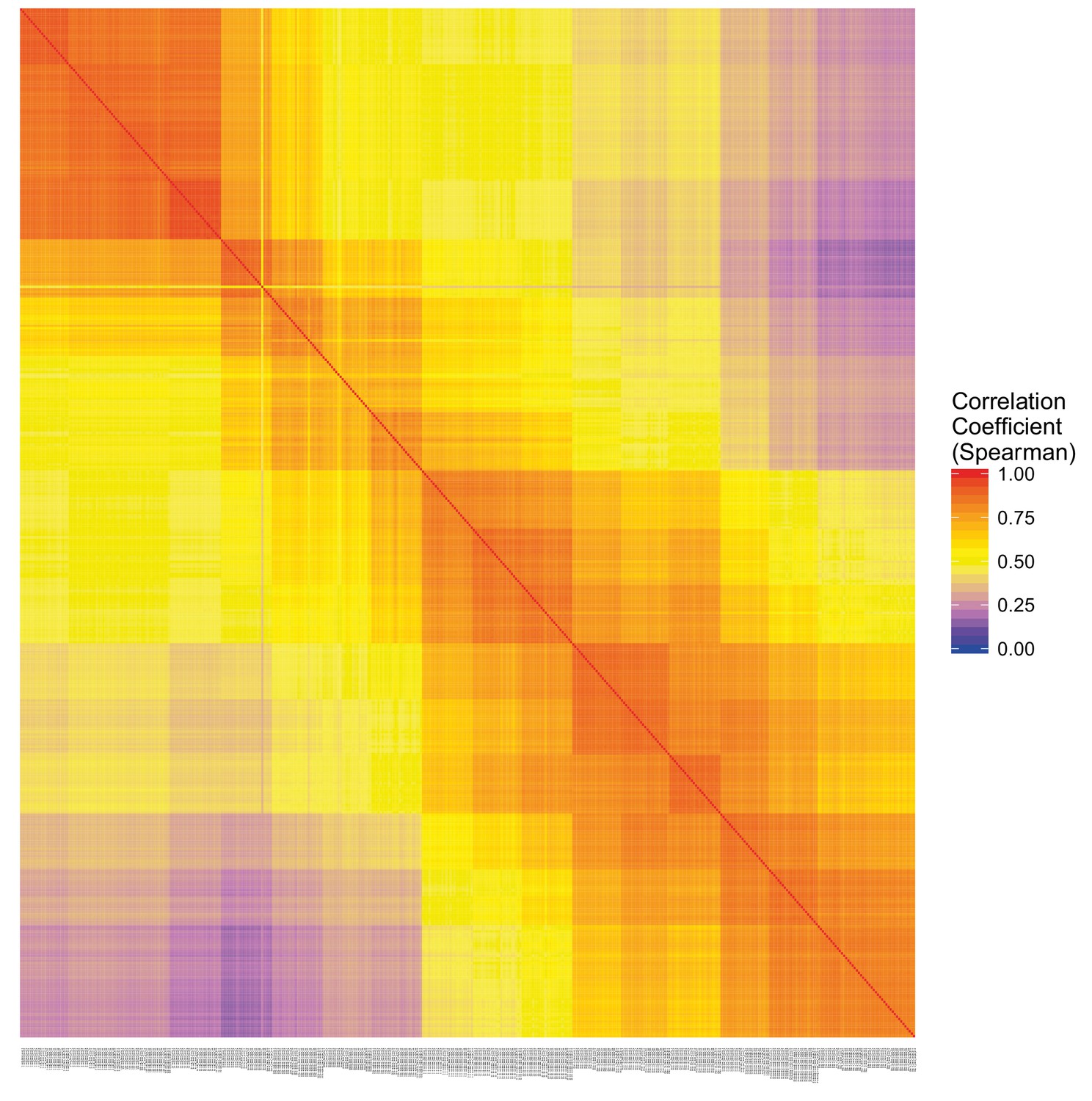
(A) Stages represented in this study. The colour scheme is used throughout the figures. Also shown are the ZFS stage IDs, stage names and approximate hours post-fertilisation (at 28.5°C) for each stage and five developmental categories. (B) Sample correlation matrix of Spearman correlation coefficients of every sample compared to every other sample. (C) Example of the overlap between H3K4me3 signal and genes. Ensembl screenshot of the region occupied by *ndr2* and *lrcc20* (the direction of transcription is indicated by arrows). Included tracks are: H3K4me3-prim-6-FE (blue) – fold enrichment of H3K4me3 ChIP-seq (H3K4me3/control) at prim-6 stage, H3K4me3-dome-FE (red) – fold enrichment of H3K4me3 ChIP-seq (H3K4me3/control) at dome/30% epiboly, Prim-5 RNAseq and Dome RNAseq (grey) – alignments of RNA-seq reads. The table above shows the genome-wide overlap between H3K4me3 ChIP-seq peaks and the promoters of expressed/not expressed genes as well as the average expression (TPM) of each gene at each stage. *ndr2* is expressed only at dome stage and displays a peak only in the dome/30% epiboly H3K4me3 ChIP-seq. *lccr20* is expressed at both stages and has a H3K4me3 peak at both stages. (D) 3D plot of Principal Component Analysis (PCA) showing the first three principal components (PCs), which together explain 83.8% of the variance in the data. Samples from the same stage cluster together and there is a smooth progression through developmental time (shown as dashed arrow). Samples are coloured as in (A) and are annotated with the stage categories. The amount of variance explained by each PC is indicated on each axis. (E) Representation of the expression profiles that contribute most to the first 6 PCs. The expression values are centred and scaled for each gene for the 100 genes that contribute most to that PC and then the mean value for each sample is plotted.

https://doi.org/10.7554/eLife.30860.002

Figure 1—figure supplement 1

Download asset Open asset

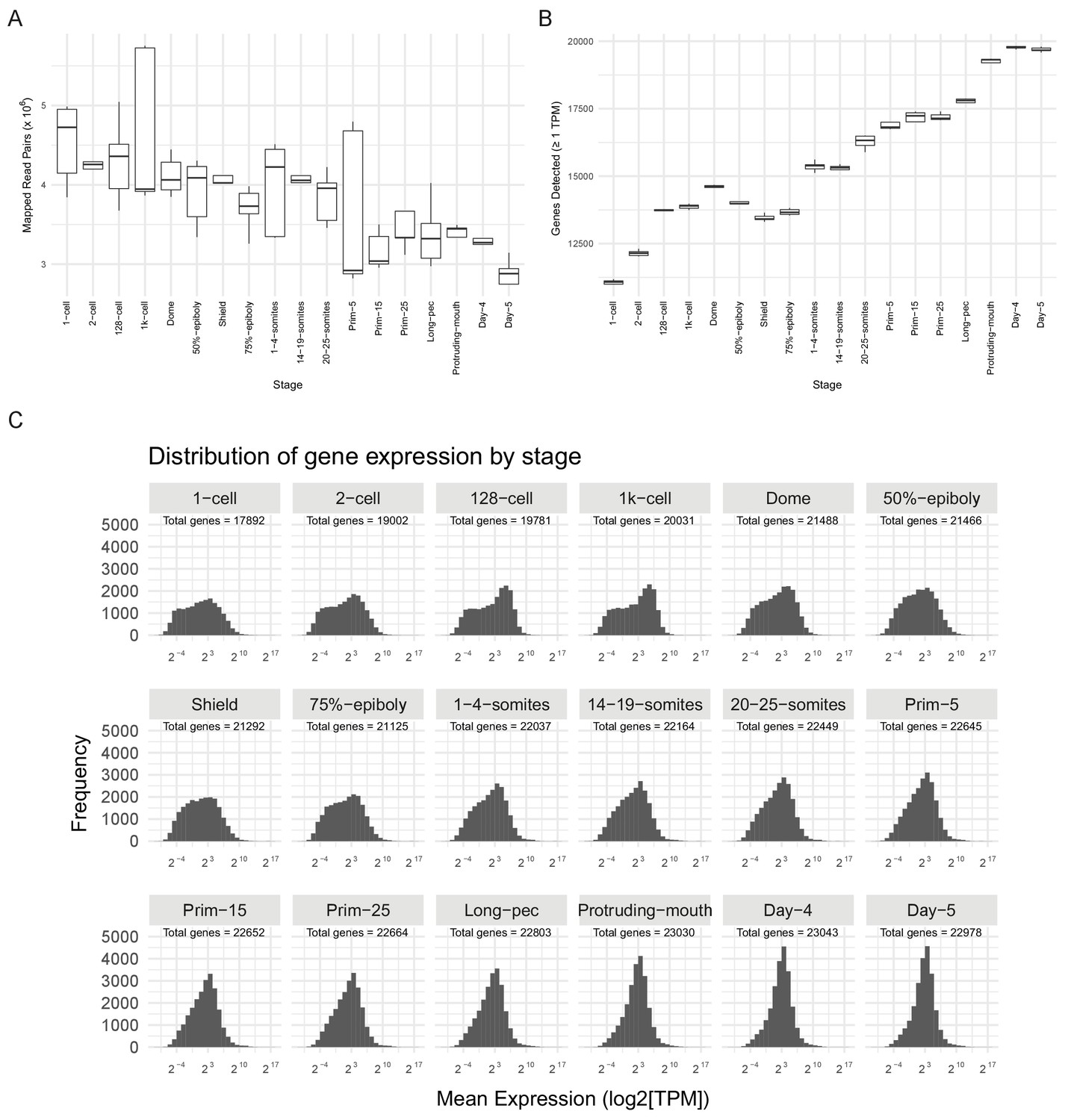
RNA-seq sample QC.

(A) Boxplot of the distributions of numbers of mapped read-pairs for each stage. (B) Boxplot of the distributions of numbers of genes detected in each sample for each stage (≥1 TPM). (C) Histograms of the distribution of gene expression levels (log2[mean TPM]) at each stage. The total number of genes represented for the stage is shown on each panel (>0 TPM for all samples at that stage). At early stages, the distribution is bimodal and shifts to unimodal as development proceeds.

https://doi.org/10.7554/eLife.30860.003

Figure 1—figure supplement 2

Download asset Open asset

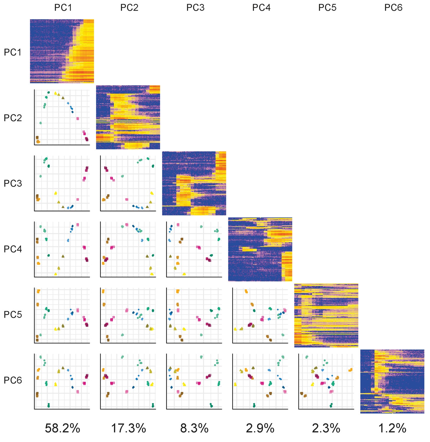
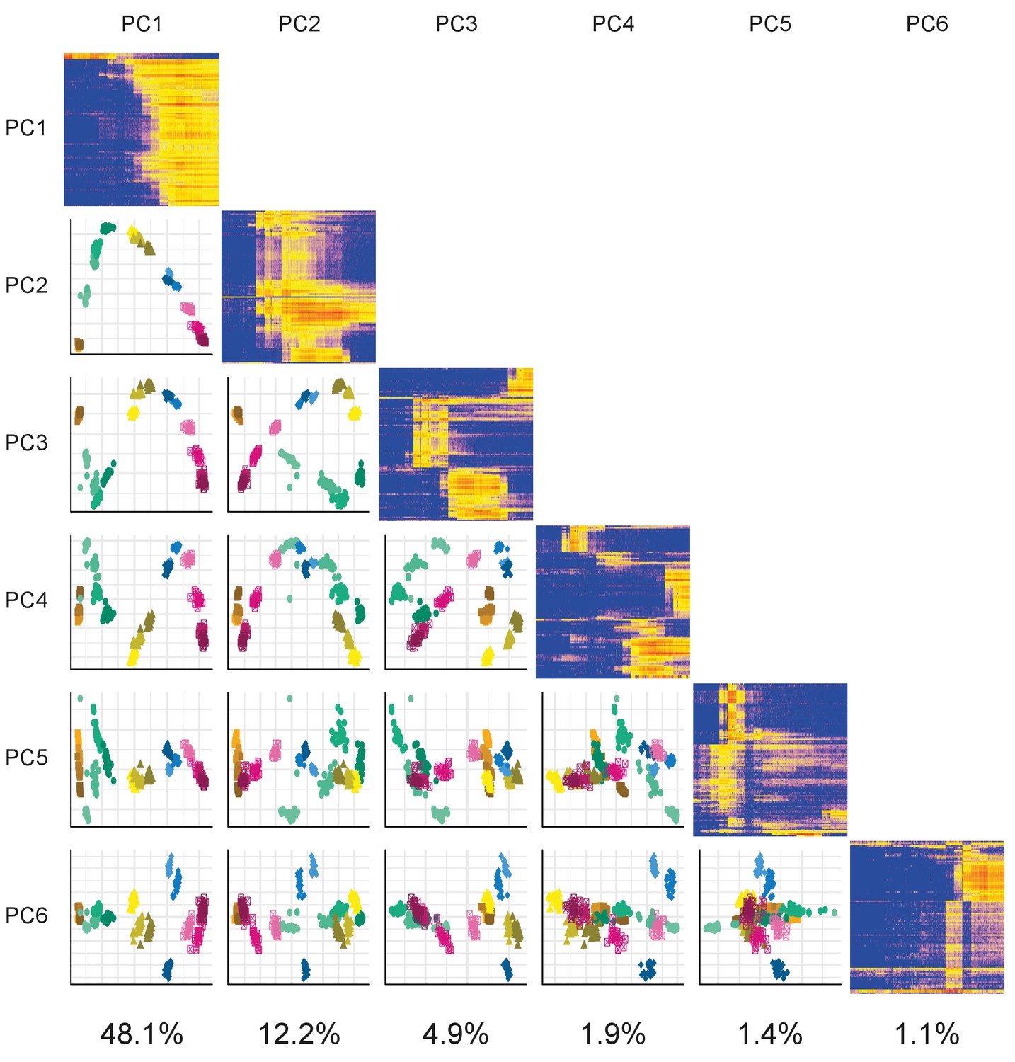
PCA matrix plot.

Plots of the first six principal components (PCs) plotted against each other. The components are arranged in a matrix from PC1 (top and left) to PC6 (bottom and right). The plots on the diagonal show the expression profiles of the 100 genes contributing the most to that component. The plots below the diagonal are the appropriate PCs plotted against each other. For example, the plot in the third row and first column is PC1 (x-axis) plotted against PC3 (y-axis). The percentage of variance explained by each PC is given underneath each column.

https://doi.org/10.7554/eLife.30860.004

Figure 2

Download asset Open asset

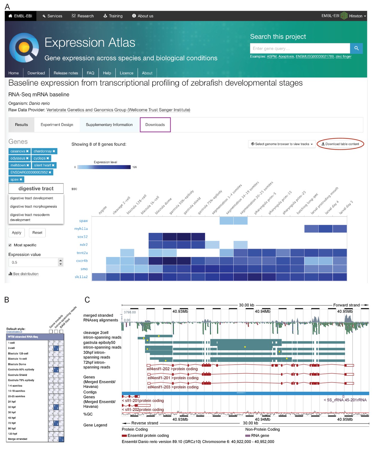
Data access.

(A) A screenshot from Expression Atlas release May 2017. Relative gene expression levels (FPKM) across all 18 stages are displayed as a heatmap. Genes can be searched for using Ensembl IDs, gene/allele names and Gene Ontology terms. The data for the selected genes can be downloaded (red ellipse) and the entire dataset can be downloaded from the ‘Downloads’ tab (purple rectangle) as either a .tsv or .Rdata file. (B) A screenshot of the RNA-seq matrix (Ensembl v89) with four intron tracks plus the exon read coverage from the merged (all 18 stages) RNA-seq data chosen for display. (C) A screenshot of the Ensembl v89 browser showing the region surrounding the gene *eif4enif1* (chr 6:40.922–40.952 Mb). Exon read coverage from the merged 18 stages is displayed as grey histograms. Four of the 18 intron-defining tracks from the RNA-seq matrix are selected. Introns are coloured in teal. Yellow dots indicate introns identifying a splice variant not found in any of the three gene models shown in red. Note that only the forward strand is shown in full and a gene model overlaps on the reverse strand.

https://doi.org/10.7554/eLife.30860.005

Figure 3 with 1 supplement

Download asset Open asset

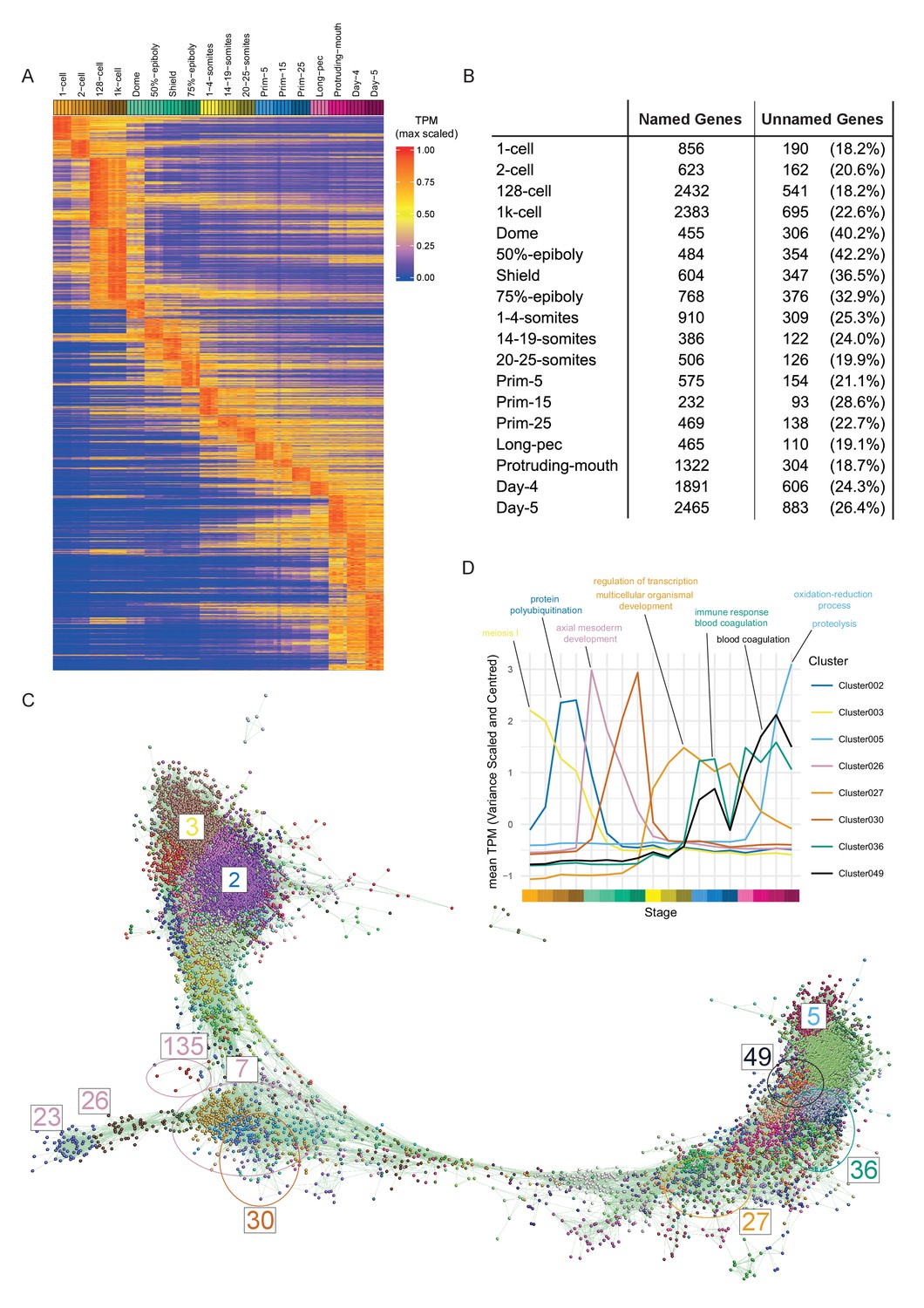
Clustering of expression patterns.

(A) Heatmap of the expression profiles across the time course (includes genes expressed at >0 TPM in all the samples for at least one stage). The expression values are scaled to the maximum expression for that gene across the time course. Genes are organised by which stage the maximum expression occurs at and clustered within each stage. (B) Table of the numbers of named and unnamed genes assigned to each stage. (C) Network diagram of the clustering produced by MCL on a network graph generated by linking genes with a Pearson correlation coefficient of >0.94 and removing unassigned genes and clusters with five genes or fewer. The numbers indicate the positions in the network diagram of the clusters shown in D and Figure 4. (D) Example clusters illustrating the progression of expression peaks through development displayed as the mean of mean-centred and variance-scaled TPM for the genes in the clusters.

https://doi.org/10.7554/eLife.30860.006

Figure 3—figure supplement 1

Download asset Open asset

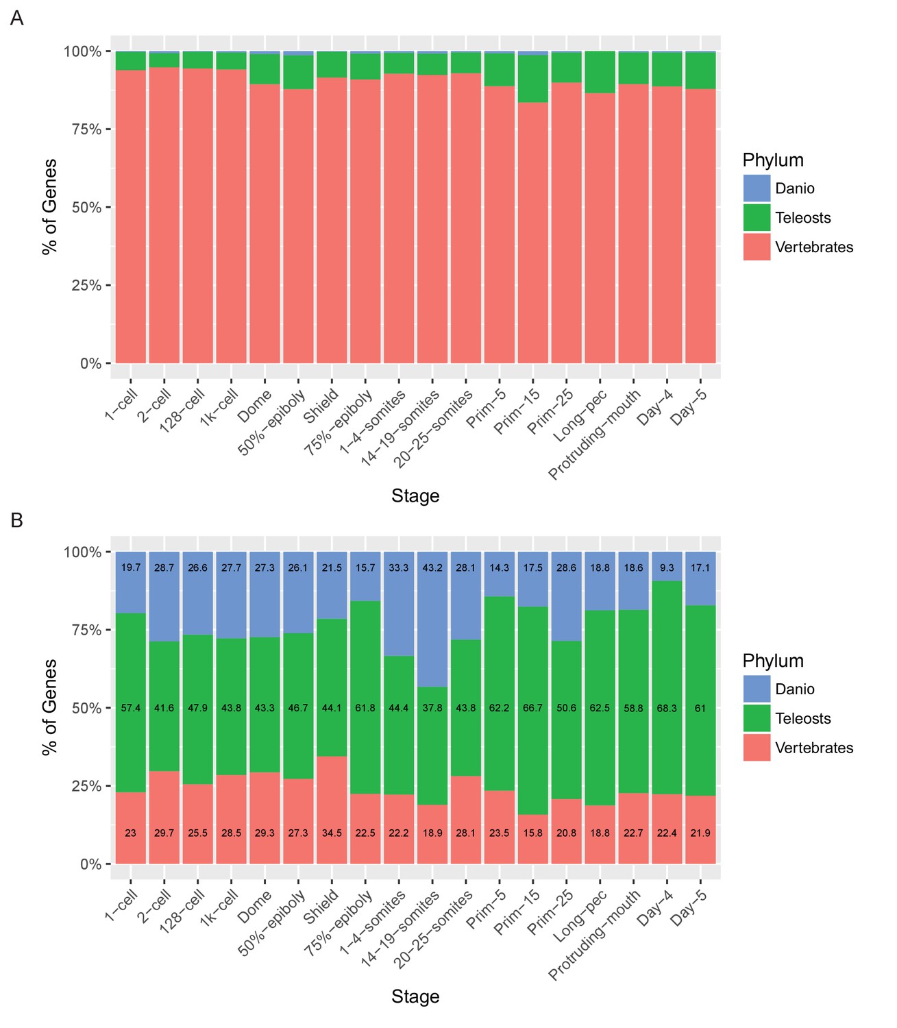
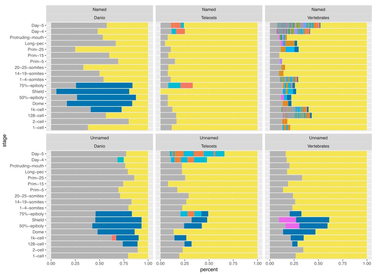
Relationship of named and unnamed genes to other species.

Stacked bar charts of the proportions of genes with orthologues at different taxonomic levels for Named (A) and Unnamed (B) genes. Orthologues for genes were obtained from the Ensembl Compara database and genes were then categorised based on the most basal Last Common Ancestor supplied by Ensembl for the orthologues. Genes with no identifiable orthologue in any of the species examined were classed as *Danio* specific (top bar, blue). Those with orthologues in the six fish species examined (*Astyanax mexicanus*, *Gasterosteus aculeatus*, *Oryzias latipes*, *Takifugu rubripes*, *Tetraodon nigroviridis*, *Gadus morhua*), but not the mammals examined were labelled Teleosts (middle bar, green). Those with orthologues also present in the mammals surveyed (*Mus musculus*, *Rattus norvegicus* and *Homo sapiens*) were labelled Vertebrates (bottom bar, red).

https://doi.org/10.7554/eLife.30860.007

Figure 4 with 1 supplement

Download asset Open asset

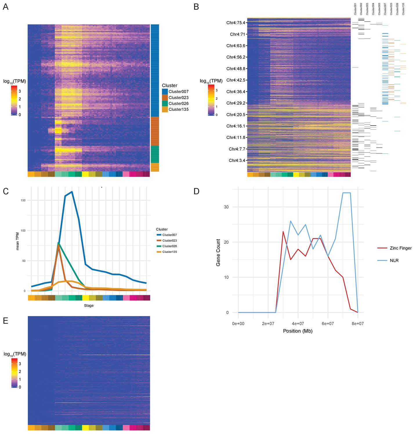
Zinc Finger (ZnF) genes expressed at the onset of zygotic transcription.

(A) Heatmap of the expression profiles (log₁₀[TPM]) of the ZnF genes from clusters 7, 23, 26 and 135. (B) Heatmap of the expression of all genes on chromosome 4 (log₁₀[TPM]) in chromosomal order with cluster assignments shown on the right. (C) Expression profiles of clusters 7, 23, 26 and 135 shown as average expression (mean TPM). (D) Plot of the distribution of ZnF (red) and NLR (blue) genes on chromosome 4. (E) Heatmap of the expression profiles (log₁₀[TPM]) of the NLR genes present in GRCz10.

https://doi.org/10.7554/eLife.30860.009

Figure 4—figure supplement 1

Download asset Open asset

Comparison of ZnF and NLR genes on chromosome 4.

The genes on chromosome 4 from 24 Mb (bottom) to the end of the chromosome (top) are displayed showing the Pearson correlation coefficient (Pearson Correlation Matrix) and expression profiles (Expression Heatmap). The Category strip on the left indicates which type each gene is (ZnF, NLR or other) and the Cluster strip shows which BioLayout cluster the genes are assigned to. The ZnF genes correlate with each other, but not with the other types of genes.

https://doi.org/10.7554/eLife.30860.010

Figure 5 with 1 supplement

Download asset Open asset

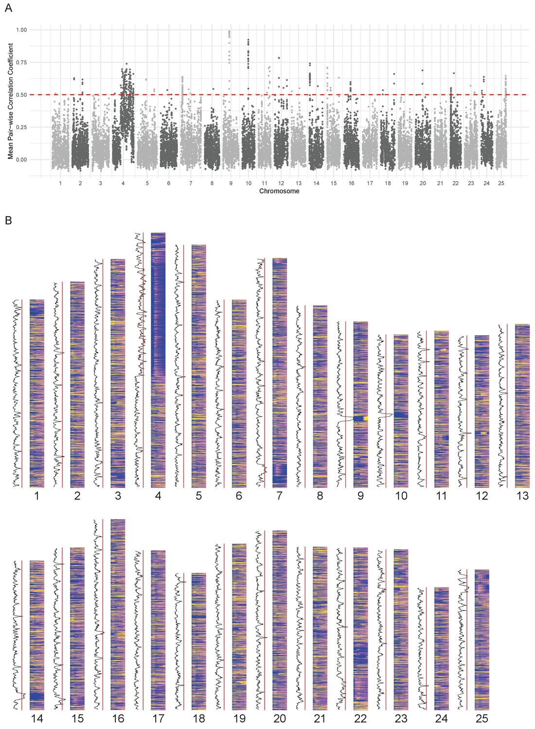
Chromosomal expression domains.

(A) Manhattan plot of the calculated similarity measure (mean pairwise Pearson correlation coefficient) in windows of 10 genes across the genome. (B) Heatmaps of the expression profiles (log₁₀[TPM]) of genes in chromosomal order. To the left of each histogram, the similarity measure is plotted as a line graph with a red line marking the 0.5 cut-off for identifying regions of co-expression.

https://doi.org/10.7554/eLife.30860.011

Figure 5—figure supplement 1

Download asset Open asset

Heatmaps showing the expression profiles of example regional expression domains.

(**A–D**) Three more regions of zinc finger genes on chromosomes 3, 15 and 22. (E) A region on chromosome 12 containing an expansion of the cathepsin L gene.

https://doi.org/10.7554/eLife.30860.012

Figure 6 with 1 supplement

Download asset Open asset

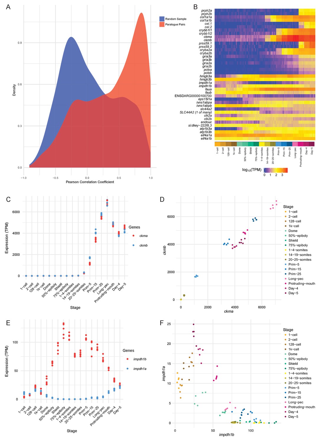
Conservation/divergence of paralogous genes.

(A) Plot of the distribution of Pearson correlation coefficients among one-to-one paralogous gene pairs (red) and a random sample of gene pairs of the same size (blue). (B) Heatmap of the expression of the gene pairs with the top 10 highest correlation coefficients (top half) and the top 10 most negative correlation coefficients (bottom half). (**C–D**) Plots displaying the expression of *ckma/b* by stage (C) and plotted against each other (D). (**E–F**) Plots showing the expression of *impdh1a/b* by stage (E) and plotted against each other (F).

https://doi.org/10.7554/eLife.30860.013

Figure 6—figure supplement 1

Download asset Open asset

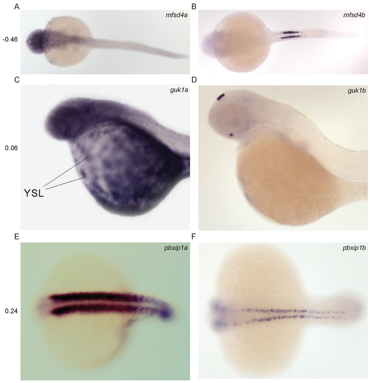
Divergent expression of paralogous pairs.

Images from ZFIN (ZFIN.org) of examples of paralogous gene pairs with diverged expression patterns. The Pearson correlation coefficient between the RNA-seq expression profiles of each pair is shown to the left. (**A–B**) *mfsd4a* (ENSDARG00000023768, ZDB-IMAGE-041130–790) and *mfsd4b* (ENSDARG00000008263, ZDB-IMAGE-060810–3118). (**C–D**) *guk1a* (ENSDARG00000030340, ZDB-IMAGE-020816–64) and *guk1b* (ENSDARG00000005776, ZDB-IMAGE-060216–46). (**E–F**) *pbxip1a* (ENSDARG00000071015, ZDB-IMAGE-020919–1927) and *pbxip1b* (ENSDARG00000011824, ZDB-IMAGE-050208–1397).

https://doi.org/10.7554/eLife.30860.014

Figure 7 with 2 supplements

Download asset Open asset

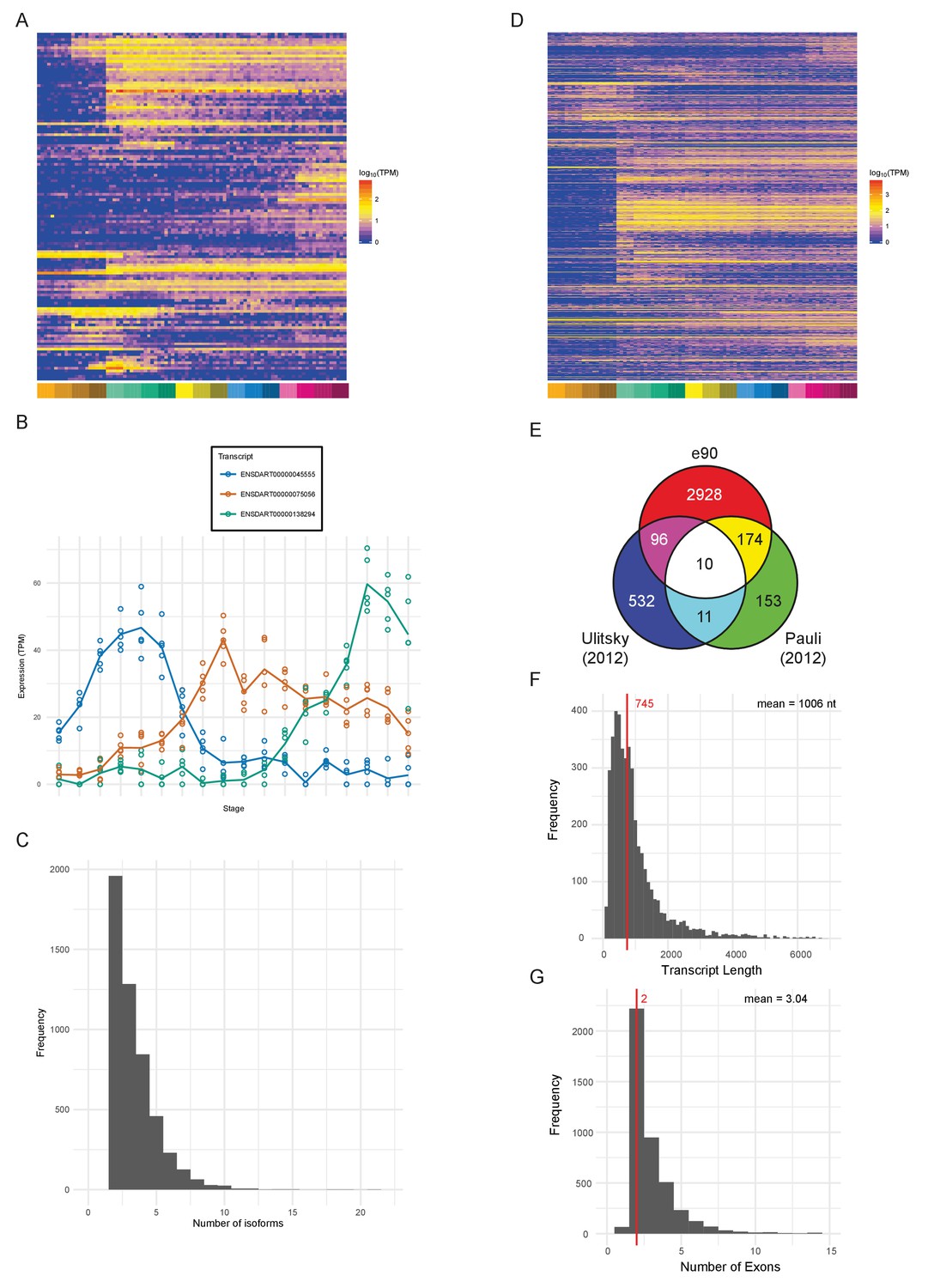
Novel features of the dataset.

(A) Heatmap of the expression profiles (log₁₀[TPM]) of the 127 new protein-coding gene annotations in the Ensembl v90 gene build produced by the contribution of this RNA-seq dataset. (B) Example of a gene (ENSDARG00000029885, *rab41*) with differential isoform usage across the time course plotted as TPM (points are individual samples and the line represents the mean). (C) Histogram of the number of isoforms per gene for genes with differentially expressed isoforms. (D) Heatmap of the expression profiles (log₁₀[TPM]) of the 1304 detected new lincRNA annotations. (E) Venn diagram showing the number of lincRNA regions that overlap with previously published lincRNA sets (Pauli et al., 2012; Ulitsky et al., 2011). (F) Histogram of the lincRNA transcript lengths. (G) Histogram of the numbers of exons per lincRNA. The red line represents the median and the mean is shown at the top right.

https://doi.org/10.7554/eLife.30860.016

Figure 7—figure supplement 1

Download asset Open asset

Differential isoform usage.

A screenshot from the Ensembl browser (v89) for the region 14:32,938,000–32,957,250. Three tracks at the top show RNA-seq coverage data (grey) for three different stages (1 k-cell, 20–25 somites and 5dpf). Orange boxes indicate the exons that change between transcripts. The three annotated transcripts are displayed below the Contigs bar. Below that are three tracks depicting intron-spanning reads defining splice events at the same three stages (the dotted arrow points to a splicing event that occurs in the 5 dpf sample, but is not represented in the 5 dpf transcript model because only the model with the most support is displayed for each stage). At the bottom are transcript models (dark blue) for all 18 time points that show the transcript model with the most support at that stage. Light blue boxes highlight the differentially-spliced exons.

https://doi.org/10.7554/eLife.30860.017

Figure 7—figure supplement 2

Download asset Open asset

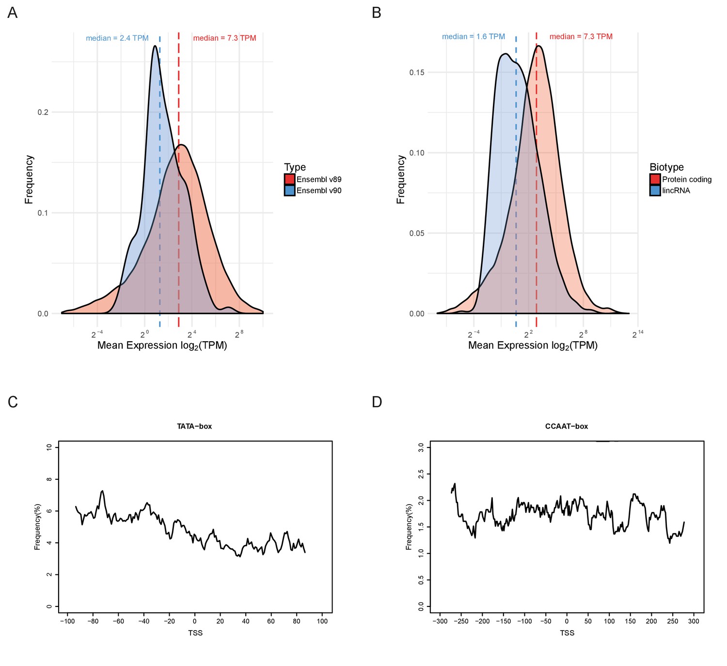
Properties of lincRNAs.

(A) Density estimates of the distributions of mean expression (mean across all samples) for the protein-coding genes present in Ensembl v89 (red) and the 127 new ones in Ensembl v90 (blue). (B) Distribution of mean expression for all protein-coding genes (red) compared to lincRNAs (blue) in Ensembl v90. (**C–D**) Frequency distributions around the predicted transcription start site of the lincRNAs from Ensembl v90 for two promoter-associated motifs. (C) TATA-box. (D) CCAAT-box.

https://doi.org/10.7554/eLife.30860.018

Figure 8

Download asset Open asset

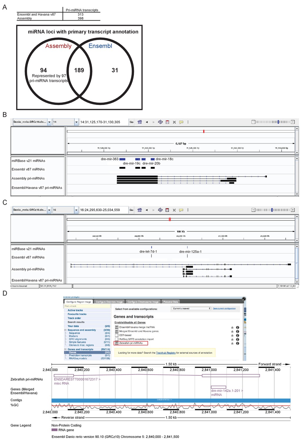
Annotation of primary miRNA transcripts.

(A) Table and Venn diagram of the numbers of assembled pri-miRNA transcripts and the overlap of Ensembl miRNAs with an annotated pri-miRNA. (**B–D**) A selection of miRNA loci for which pri-miRNA annotation is not available in Ensembl and Havana v87. (**B–C**) IGV screen shots illustrating the assembled pri-miRNA transcripts overlapping mir-363, mir-19c, mir-20b and mir-18c (B), and mir-125 (C). Tracks shown are miRNA annotations from miRBase and Ensembl, newly assembled pri-miRNA transcripts and Ensembl pri-miRNAs. (D) Screen shots from the Ensembl v90 browser demonstrating how to display the pri-miRNAs. The track is selectable from the ‘Genes and transcripts’ section of the ‘Configure this page’ menu. The region around miR-142a (chr5: 2,840,000–2,841,500) is shown with its annotated pri-miRNA.

https://doi.org/10.7554/eLife.30860.019

Figure 9 with 3 supplements

Download asset Open asset

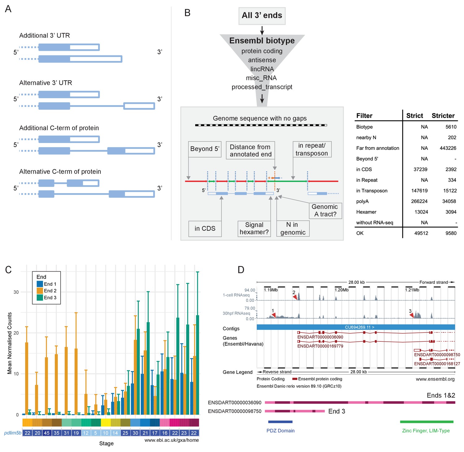
Alternative 3’ end use during development.

(A) Diagrams illustrating the possible outcomes of differential 3’ end usage. Only the 3’ end of the gene is shown, where the exons are boxes, the introns are represented as lines and filled boxes are coding. The dotted line represents the remaining 5’ end of the gene. (B) Flowchart of the DeTCT 3’ end filtering strategy. See Materials and methods for the definition of each filter. The table shows the number of ends removed by each filter when using the strict/stricter settings. (C) Graph of the mean normalised counts by stage for the three alternative 3’ ends (shown in D) of the *pdlim5b* gene. Error bars represent standard deviations. Underneath is a screenshot from Expression Atlas (Aug 2017) showing the overall TPM for *pdlim5b*. (D) Screenshot from Ensembl (release 89) showing the 3’ portion of the *pdlim5b* gene (10:1,187,000–1,215,000). The top two tracks are RNA-seq coverage for 1 cell and prim-15 (30 hpf). Red arrowheads point to the genomic positions of the three transcript ends. Note, the 3’ UTR resulting in end 1 is not annotated in this genebuild. Below is a schematic of the proteins that are predicted to be produced by two of the transcripts. The positions of domains within the protein are also indicated.

https://doi.org/10.7554/eLife.30860.020

Figure 9—figure supplement 1

Download asset Open asset

DeTCT QC.

Sample correlation matrix of the Pearson correlation coefficient between each pairwise comparison of samples.

https://doi.org/10.7554/eLife.30860.021

Figure 9—figure supplement 2

Download asset Open asset

DeTCT PCA.

DeTCT Matrix PCA plot. Plot showing the PCA of the DeTCT data arranged in the same way as Figure 1—figure supplement 2.

https://doi.org/10.7554/eLife.30860.022

Figure 9—figure supplement 3

Download asset Open asset

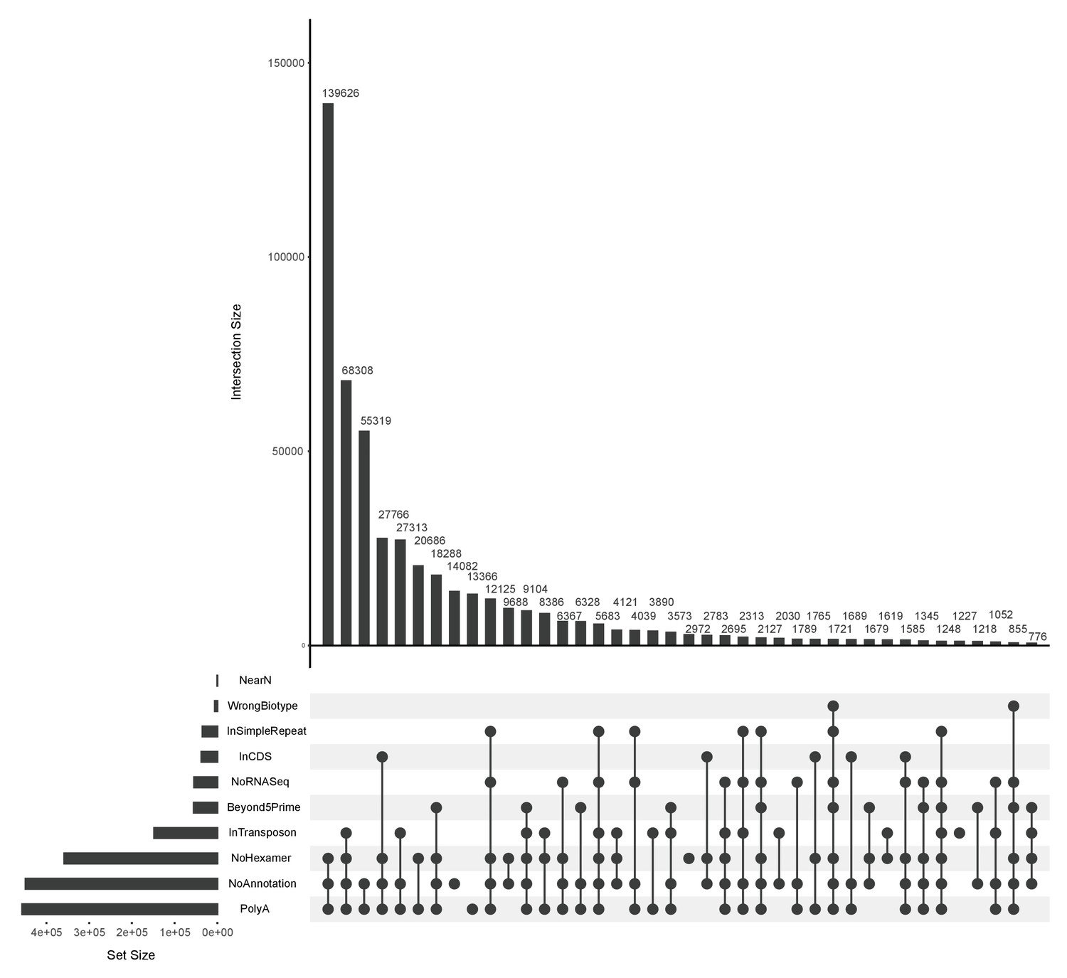
3’ end filtering.

UpSet (Conway et al., 2017) plot showing the overlap of the ends that fail different 3’ end filtering rules (stricter). Underneath the main bar chart are the different filters and the filled circles indicate the particular overlap displayed in the bar above. The height of the bar above shows the size of that overlap set. For example, the first bar in the main bar chart shows that 139,626 ends failed all three of the No Hexamer, No Annotation and PolyA filters. The horizontal bar chart to the left displays the size of the set for individual filters.

https://doi.org/10.7554/eLife.30860.023

Author response image 1

Download asset Open asset

Gene detection with reads downsampled to 2 million read pairs per sample.

Author response image 2

Download asset Open asset

Comparison of genes detected from one stage to the next.

Author response image 3

Download asset Open asset

Tables

Table 1

BioLayout clusters with significant chromosomal enrichments (adjusted p-value<0.05 and log₂ fold enrichment [log₂FE]>1).

https://doi.org/10.7554/eLife.30860.008

Cluster	Chromosome	Count	Expected	log₂[FE]	Adjusted p-value
Cluster007	Chr4	99	23.55	2.07	4.772e-35
Cluster023	Chr4	40	6.11	2.71	2.707e-23
Cluster026	Chr4	20	5.03	1.99	1.810e-06
Cluster135	Chr4	9	0.99	3.19	6.997e-07
Cluster086	Chr12	7	0.42	4.05	3.447e-06
Cluster057	Chr23	6	0.69	3.13	1.637e-03

Table 2

Comparison of Ensembl genebuild versions 89 and 90.

https://doi.org/10.7554/eLife.30860.015

Biotype	e89	e90
protein_coding	25,672	25,743
snRNA	1287	1287
processed_transcript	1106	1106
lincRNA	914	3208
rRNA	780	1579
miRNA	767	440
antisense_RNA	696	696
snoRNA	297	305
unprocessed_pseudogene	228	228
Other	519	525
Total Genes	32,266	35,117
Total Transcripts	58,549	62,895

Key resource table

Reagent type (species) or resource	Designation	Source or reference	Identifiers	Additional information
genetic reagent (Danio rerio)	drosha^sa191	this paper	ZFIN:sa191; RRID: ZFIN_ZDB-ALT-100831-1	ENU mutant. C - > T at position GRCz10:12:13311049. Available from ZIRC (http://zebrafish.org/fish/lineAll.php?OID=ZDB-ALT-100831-1)
genetic reagent (D. rerio)	dgcr8^sa223	this paper	ZFIN:sa223; ZFIN: ZDB-ALT-161003–11399	ENU mutant. C - > T at position GRCz10:12:24021119
strain, strain background (D. rerio)	HLF	this paper		Hubrecht Long Fin
software, algorithm	TopHat	10.1038/nprot.2012.016	RRID:SCR_013035
software, algorithm	Cufflinks	10.1038/nprot.2012.016	RRID:SCR_014597
software, algorithm	QoRTs	10.1186/s12859-015-0670-5		https://github.com/hartleys/QoRTs
software, algorithm	htseq-count	10.1093/bioinformatics/btu638	RRID:SCR_011867
software, algorithm	R	https://www.r-project.org/	RRID:SCR_001905
software, algorithm	Perl	https://perldoc.perl.org/
software, algorithm	zfs-devstages	this paper		github repository, https://github.com/richysix/zfs-devstages
software, algorithm	Ontologizer	10.1093/bioinformatics/btn250	RRID:SCR_005801
software, algorithm	STAR	10.1093/bioinformatics/bts635
software, algorithm	Samtools	10.1093/bioinformatics/btp352	RRID:SCR_002105
software, algorithm	Picard	http://broadinstitute.github.io/picard	RRID:SCR_006525
software, algorithm	gtfToGenePred	UCSC Genome Browser		http://hgdownload.soe.ucsc.edu/downloads.html#utilities_downloads
software, algorithm	genePredToBed	UCSC Genome Browser		http://hgdownload.soe.ucsc.edu/downloads.html#utilities_downloads