Targeted cortical reorganization using optogenetics in non-human primates
- University of California, San Francisco, United States
- University of Washington, United States
Figures
Figure 1 with 1 supplement
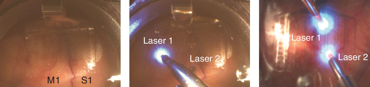
Stimulation and recording setup.
Photo of the µECoG array placement over M1 and S1 in Monkey G (left panel) and the placement of lasers on top of the array in two different configurations (middle panel: Monkey G and right panel: Monkey J).
Figure 1—figure supplement 1

Opsin expression was observed only in pyramidal neurons.
Using immunohistochemistry, we confirmed that EYFP reporter expression was present in both S1 and M1. YFP-positive cells in these areas were morphologically identified as pyramidal neurons, and were in layers II-III, V-VI. To confirm this we further analyzed the tissue using markers for inhibitory neurons such as parvalbumin, somatostatin and calbindin as well as GAD67/65 and examined cell bodies and axonal terminals at the areas around the site of infusion. We found no evidence for co-localization between EGFP and any of the inter-neuronal markers therefore excluding the possibility for significant opsin presence in cells other than pyramidal neurons, and confirmed that optical stimulation was selectively activating excitatory pyramidal neurons in M1 and S1. (A) Low magnification image of the coronal section processed anti-GFP antibody showing the medio-lateral aspect of YFP expression in the somatosensory cortex of monkey J (areas 1, 2, 3). The black arrowhead indicates the location of the injector needle track; the adjacent tissue (black frame) is microscopically enlarged in B to show laminar distribution of the YFP-positive cells. In monkey G (Yazdan-Shahmorad et al., 2016), we saw some cortical thinning post-mortem. In contrast, the histology for monkey J, presented here does not show change in the cortical thickness. (B) Densely YFP-positive cells are located predominantly in layers II-III and V-VI, and also show typical pyramidal morphology (cells in white frames are further enlarged in panels C-E). White arrowheads on bottom panels C-E point to typical pyramidal cells in layers II-III (C); layer V (D); and layer VI (E). Scale bars: A, 2 mm; B, 200 μm; C-E, 100 μm. (F) Stained parvalbumin neurons (red) and YFP-expressing cells (green), no overlap indicated high specificity. Scale bar: 30 μm.
Figure 2
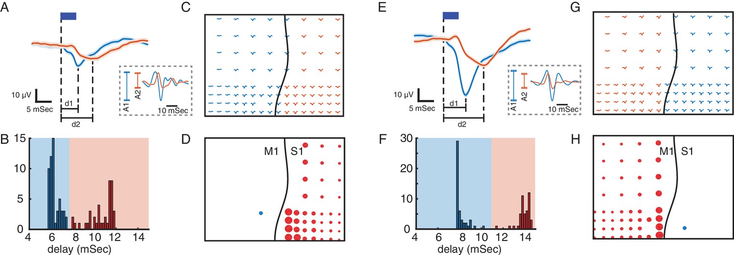
Using evoked responses to measure connectivity across M1 and S1.
(A) Primary (blue) and secondary (orange) evoked responses to light stimulation. The dark blue rectangle represents the duration of light stimulation. Shaded areas show standard error. The delays of evoked responses are calculated as the time difference between the onset of stimulation and the time of the response trough (vertical lines at d1 and d2). (B) Distribution of the delays color-coded based on the primary and secondary light-evoked responses. (C) Evoked responses across the array, color-coded based on the delays. As shown here there is a spatial separation of primary and secondary responses that corresponds to the locations of M1 and S1. This suggests that due to functional connectivity between M1 and S1, we see a delayed (secondary) response in S1 to light stimulation in M1. (D) S1 connectivity with the site of stimulation. The blue circle shows the location of stimulation in M1. The black line shows the location of central sulcus with respect to the recording array. The size of the red circles represents the strength of connectivity between each site and the stimulation location for the recording sites with secondary responses across S1. SERR Connectivity is defined as the peak-to-trough of filtered high gamma responses (60–200 Hz: trace plots shown on the dashed rectangle on A) at each site (orange) normalized to the peak-to-trough of high gamma at the site of stimulation (blue). (E–H) Same as A-D with the same array placement and S1 stimulation.
Figure 3
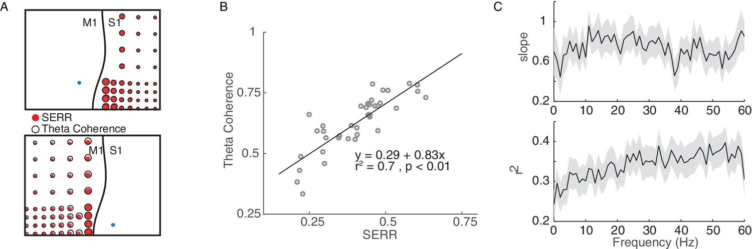
Coherence measure of inter-area connectivity correlates with SERR.
(A) S1 (Top panel) and M1 (bottom panel) theta coherence and SERR connectivity with the site of stimulation in monkey G. The blue circle shows the location of stimulation. The black line shows the location of central sulcus with respect to the recording array. The size of the red and white circles represents the strength of connectivity between each secondary site and the stimulation location. (B) An example session showing relationship between SERR and theta coherence. The black line shows the linear regression fit. (C) Linear relationship between evoked response and coherence across different frequencies. Summary data showing the mean and standard error (shaded region) of regression parameters (shown in B) across frequencies.
-
Figure 3—source code 1
Comparing SERR and coherence measurements for example session and across sessions.
- https://doi.org/10.7554/eLife.31034.007
-
Figure 3—source data 1
SERR and coherence across channels for example session and across sessions.
- https://doi.org/10.7554/eLife.31034.008
Figure 4 with 2 supplements
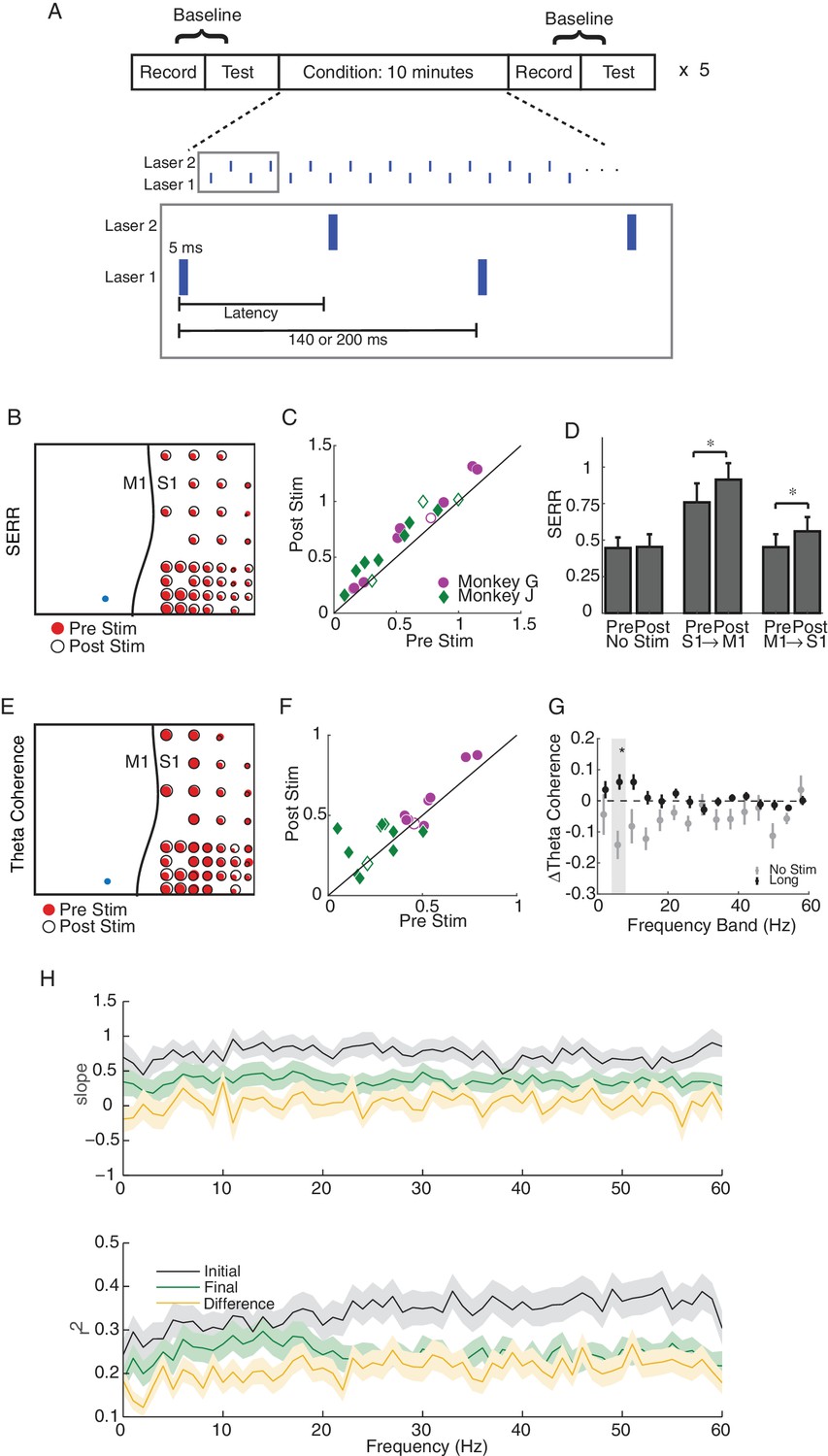
Single site and long-latency stimulation increase the functional connectivity between M1 and S1.
(A) Experimental protocol. Conditioning stimulation was interrupted by periodic connectivity measurements including passive recording and active testing. Either one or two non-interfering lasers were used. (B) Examples of changes in SERR across the recording array in monkey G. Red circles show initial connectivity and white circles show connectivity after 50 min. of conditioning. (C) Summary of SERR changes across all experiments. Each symbol represents the connectivity averaged over all secondary channels for one experiment. Filled markers show significant changes (paired t-test; p<0.05, the p-values for each experiment are listed in the supplementary spreadsheet). (D) Changes in SERR when stimulating in either S1 or M1 in comparison to control. Error bars represent standard error and asterisks show significant changes (paired t-test; Control: p=0.8, laser in S1: p=0.01, laser in M1: p=1.6e-04). (E) Examples of changes in theta (4–8 Hz) coherence across the recording array. (F) Summary of theta coherence changes across all experiments. Each marker represents the connectivity averaged over all channels for one experiment. Filled markers show significant changes (paired t-test; p<0.05, the p-values for each experiment are listed in the supplementary spreadsheet). (G) Change in coherence across different frequency bands in comparison to controls. Asterisk show significant difference between the two groups (unpaired t-test, Bonferroni corrected; p<0.05, the p-values are listed in the supplementary spreadsheet). (H) Linear relationship between SERR and coherence across different frequencies for pre-stim, post-stim and the change in both measures. Summary data showing the mean and standard error (shaded region) of regression slope and r2 as a function of coherence frequency (see the example regression for the theta-band in Figure 3B).
-
Figure 4—source code 1
Comparing SERR and coherence measurements across channels for example session and for all sessions broken down by experimental condition.
- https://doi.org/10.7554/eLife.31034.016
-
Figure 4—source data 1
SERR and coherence measurements across channels for example session and for all sessions broken down by experimental condition.
- https://doi.org/10.7554/eLife.31034.017
Figure 4—figure supplement 1

Linear relationship between SERR and coherence across different frequencies for control sessions.
Replication of Figure 4H for control (no stimulation) sessions. Each line shows the mean and standard error (shaded region) of regression slope and r2 as a function of the coherence frequency.
-
Figure 4—figure supplement 1—source code 1
SERR and coherence relationship across different frequencies for control sessions.
- https://doi.org/10.7554/eLife.31034.011
-
Figure 4—figure supplement 1—source data 1
SERR and coherence measurements acrossdifferent frequencies and channels for control sessions.
- https://doi.org/10.7554/eLife.31034.012
Figure 4—figure supplement 2
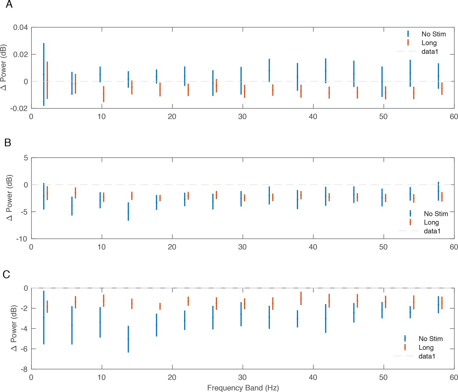
Change in power following stimulation.
Change in power from pre- to post-conditioning across monkeys and non-interference experiments. Bars reflect standard errors around the mean change in power in each 4 Hz frequency band. (A) Average change in power across secondary recording sites normalized to the change in power at the stimulation site. (B) Average change in power across secondary recording sites. (C) Average change in power at the stimulation site.
-
Figure 4—figure supplement 2—source code 1
Comparison of power measurements between control and stimulation data across different frequency bands.
- https://doi.org/10.7554/eLife.31034.014
-
Figure 4—figure supplement 2—source data 1
Power measurementsacross different frequency bands for each session.
- https://doi.org/10.7554/eLife.31034.015
Figure 5 with 1 supplement
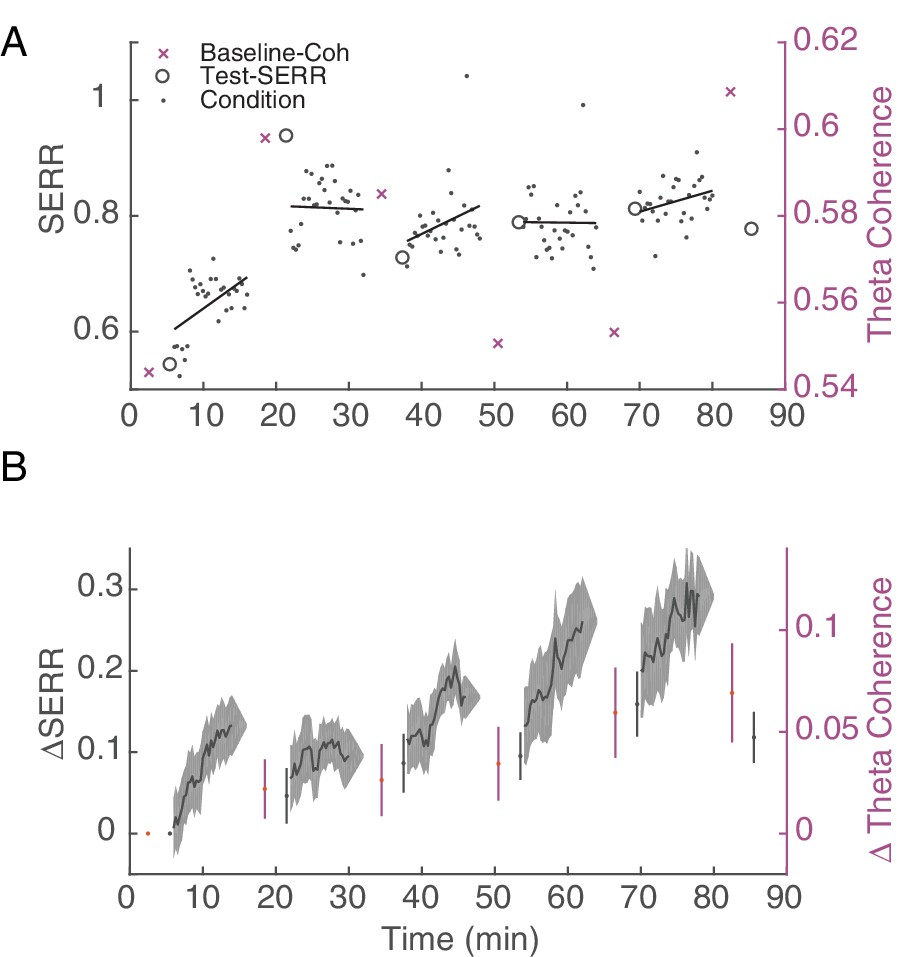
Stimulation induces an increase in inter-area connectivity across time.
(A) An example of the dynamics of mean inter-area SERR and coherence in an experiment. Black lines show linear regression to each conditioning block. (B) Dynamics of change in SERR and theta coherence with respect to baseline connectivity across all experiments (shaded area show standard error).
-
Figure 5—source code 1
Change in SERR and coherence measurements for example session and summary over stimulation sessions.
- https://doi.org/10.7554/eLife.31034.022
-
Figure 5—source data 1
SERR and coherence measurements for stimulation sessions.
- https://doi.org/10.7554/eLife.31034.023
Figure 5—figure supplement 1
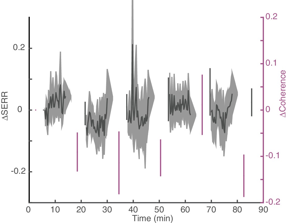
Dynamics of changes in connectivity for control sessions.
Replication of Figure 5B for control (no stimulation) sessions. Dynamics of change in SERR and theta coherence with respect to baseline connectivity across all experiments (shaded area show standard error).
-
Figure 5—figure supplement 1—source code 1
Change in SERR and coherence measurements for control sessions across time.
- https://doi.org/10.7554/eLife.31034.020
-
Figure 5—figure supplement 1—source data 1
SERR and coherence measurements for control sessions across time.
- https://doi.org/10.7554/eLife.31034.021
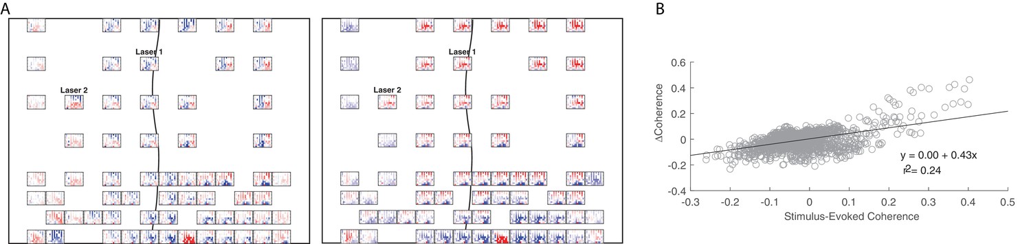
Figure 6

Hebbian plasticity models explain stimulation-induced fine-scale network connectivity changes.
(A) An example session highlighting the similarity between the stimulus-evoked coherence (middle panel) and the change in baseline coherence (left panel) across the array in Monkey J. At each recording site across the array, a heatmap represents the respective coherence between that location with all other recording sites. Enlarged examples for a single location are compared in the right panel. The black line shows the location of central sulcus on the array and rectangles show the location of the magnified examples. The average value across the array was subtracted for visualization. (B) Linear regression between stimulus-evoked coherence and the change in baseline coherence for the example session shown in A. (C) Summary of regression parameters across single-site and non-interference experiments. Errorbars show standard error.
-
Figure 6—source code 1
Comparing pairwise coherence measurements for example session and summary of regression parameters for stimulation sessions.
- https://doi.org/10.7554/eLife.31034.025
-
Figure 6—source data 1
Pairwise coherence measurements for example session and regression parameters for all sessions by experimental condition.
- https://doi.org/10.7554/eLife.31034.026
Figure 7 with 2 supplements

Hebbian plasticity models explain fine-scale network connectivity changes driven by complex spatio-temporal stimulation patterns.
(A) Same stimulation protocol as described in 4A. However, here we reduced the latency between to the two lasers to 10 ms or 30 ms, creating a more complicated pattern of stimulation. (B) An example of the stimulus-evoked activity across the array from Monkey G. Blue circles show the locations of stimulation. The inset shows the enlarged pattern of evoked response at the framed electrode, which is located close to both lasers. (C) Summary of inter-area theta coherence changes for all interference experiments across both monkeys. (D) Summary of regression parameters across all interference experiments. Errorbars show standard error.
-
Figure 7—source code 1
Coherence measurements and regression parameters for short-latency stimulation sessions.
- https://doi.org/10.7554/eLife.31034.034
-
Figure 7—source data 1
Coherence measurements and regression parameters for short-latency stimulation sessions.
- https://doi.org/10.7554/eLife.31034.035
Figure 7—figure supplement 1
Short-latency example showing the relationship between input coherence and change in baseline coherence.
(A) An example showing similarity between the input coherence (right panel) and the change in baseline coherence (left panel) in monkey J. Same as Figure 6A. (B) Linear regression between input coherence and the change in baseline coherence for the example session shown in A.
-
Figure 7—figure supplement 1—source code 1
Comparing pairwise coherence measurements for example session and regression parameters for all sessions by experimental condition.
- https://doi.org/10.7554/eLife.31034.029
-
Figure 7—figure supplement 1—source data 1
Pairwise coherence measurements for example session and regression parameters for all sessions by experimental condition.
- https://doi.org/10.7554/eLife.31034.030
Figure 7—figure supplement 2
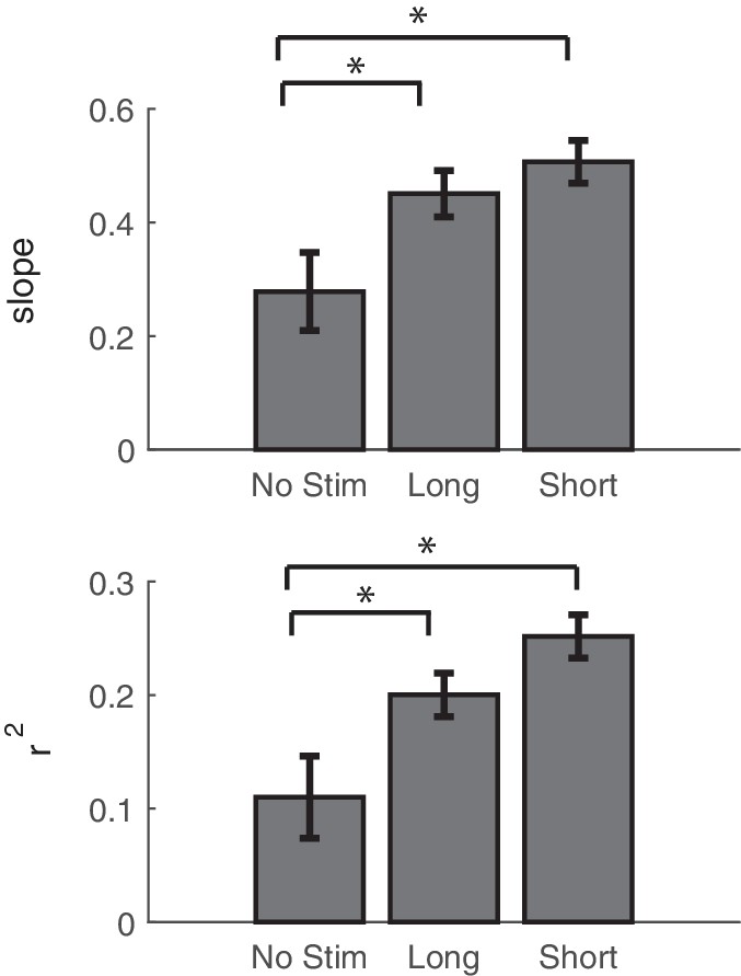
Comparing the effects of stimulation on network connectivity between stimulation and controls.
Summary of regression fits of the change in theta coherence vs. the stimulus-evoked theta coherence. Slope and r2 values are reported as averages across stimulation blocks for non-interference stimulation (also reported in Figure 6C), interference-stimulation (also reported in Figure 7D), and control sessions. Error bars show standard error.
-
Figure 7—figure supplement 2—source code 1
Plot regression parameters for all sessions by experimental condition.
- https://doi.org/10.7554/eLife.31034.032
-
Figure 7—figure supplement 2—source data 1
Regression parameters for all sessions by experimental condition.
- https://doi.org/10.7554/eLife.31034.033
Tables
Table 1
Summary of the sessions for both monkeys.
The data was collected in two to three week periods for each animal. Depending on the health of the animal and the quality of the neural recordings one to four experiments were performed per day.
| Monkey G | Monkey J | |
|---|---|---|
| Number of sessions | 37 | 33 |
| Number of sessions analyzed | 29 | 15 |
| Number of control sessions | 3 | 2 |
| Number of single-site and long latency sessions | 6 | 9 |
| Number of short-latency sessions | 20 | 4 |
Table 2
Comparison between different measures for calculating SERR.
We decided a priori to calculate the SERR using the high gamma peak to trough as a response metric, since high gamma potentials are thought to represent the population activity of local cortical columns (Yazdan-Shahmorad et al., 2013; Suzuki and Larkum, 2017). Post-hoc, we performed further analysis to investigate whether the other measures (listed in the above table) show similar effects to the high-gamma peak to trough. As shown here, all of the measures show a significant increase following stimulation (second column) whereas they do not show a significant change after control sessions in which there is no stimulation applied (first column). However, other measures are more variable and do not show increases relative to the control sessions (third column). Furthermore, only high-gamma peak to trough and broadband amplitude are significantly correlated with coherence in the baseline condition (fourth column). Overall, this suggests that the amplitude of the high-gamma signal is the best of these metrics for estimating connectivity. All effect sizes in this table reflect the median change in connectivity across sessions for each measure; p-values reflect the output of signrank (columns 1 and 2) and ranksum (column 3) statistical tests.
| Evoked Response Measure | Change in Connectivity during Control Sessions | Change in Connectivity during Long Latency Stim Sessions | Change in Connectivity in Control Sessions Vs. Change in Connectivity in Stim Sessions | Correlation Between Coherence (Across Freqs) and Evoked Response Connectivity Measure |
|---|---|---|---|---|
| high-gamma peak to trough (SERR) | eff_size = 0.018 p=1.0 | eff_size = 0.118 p=1.6e-04 | eff_size = 0.100 p=6.6e-03 | avg_slope = 0.57 p=3.7e-06 |
| high-gamma energy | eff_size = 0.09 p=0.38 | eff_size = 0.86 p=3.3e-03 | eff_size = 0.77 p=0.184 | avg_slope = 0.037 p=0.144 |
| broadband energy | eff_size = 0.28 p=0.22 | eff_size = 0.39 p=5.4e-04 | eff_size = 0.12 p=0.386 | avg_slope = −0.02 p=0.652 |
| broadband amplitude | eff_size = 0.21 p=0.30 | eff_size = 0.23 p=4.6e-04 | eff_size = 0.01 p=0.184 | avg_slope = 0.183 p=0.002 |
| broadband slope | eff_size = 0.09 p=0.22 | eff_size = 0.23 p=4.6e-04 | eff_size = 0.13 p=0.184 | avg_slope = 0.028 p=0.318 |
-
Table 2—source code 1
Statistics of SERR and other connectivity measures for each session in each experimental condition.
- https://doi.org/10.7554/eLife.31034.038
-
Table 2—source data 1
SERR and other connectivity measures for each session in each experimental condition.
- https://doi.org/10.7554/eLife.31034.039
Additional files
-
Supplementary file 1
Spreadsheet of statistical information
- https://doi.org/10.7554/eLife.31034.040
-
Transparent reporting form
- https://doi.org/10.7554/eLife.31034.041
Download links
A two-part list of links to download the article, or parts of the article, in various formats.
Downloads (link to download the article as PDF)
Open citations (links to open the citations from this article in various online reference manager services)
Cite this article (links to download the citations from this article in formats compatible with various reference manager tools)
Targeted cortical reorganization using optogenetics in non-human primates
eLife 7:e31034.
https://doi.org/10.7554/eLife.31034


